
Analysis of Compositions of Microbiomes with Bias Correction (ANCOM-BC)
Source:R/ancombc.r
ancombc.RdEstimates each feature's log fold change for every covariate of a linear
model, corrected for the bias that differing sampling fractions cause,
with standard errors and p-values (Lin & Peddada 2020, 2024).
ancombc() is ANCOM-BC; ancombc2() is ANCOM-BC2, which also corrects
each sample's logs for its estimated sampling fraction before refitting,
adds a variance floor for rare features, uses t tests, and by default
treats zeros as missing values instead of adding a pseudocount. Both
follow scikit-bio's ancombc() and ancombc2().
Usage
ancombc(
  counts,
  formula = NULL,
  data = NULL,
  groups = NULL,
  margin = 1L,
  pseudocount = NULL,
  max_iters = 100L,
  tol = 1e-05,
  alpha = 0.05,
  p_adjust = "holm",
  sensitivity = FALSE,
  cpus = n_cpus()
)

ancombc2(
  counts,
  formula = NULL,
  data = NULL,
  groups = NULL,
  margin = 1L,
  pseudocount = 0,
  var_quantile = 0.05,
  max_iters = 100L,
  tol = 1e-05,
  alpha = 0.05,
  p_adjust = "holm",
  sensitivity = TRUE,
  cpus = n_cpus()
)
Arguments
- counts
A numeric matrix of non-negative abundances (samples \(\times\) features), or any of the objects listed under Input Types. Counts, proportions, and the output of
replace_zeros()are all accepted: each sample's scale is absorbed by its sampling fraction.- formula
The model, a one-sided formula over the columns of
data, such as~ status + age, or the same as a string ('status + age', with or without the~). Anythingstats::model.matrix()accepts may be used, including interactions (status * age) and a model without an intercept (~ 0 + status). Every factor is coded with treatment contrasts (see Covariates).NULL(the default) is~ groups: giveformula,groups, or both.- data
A data frame of sample metadata, with the variables of
formula. Its rows are matched to the samples ofcountsby name when both have names (rows for other samples are left out), else by position. A single vector or factor is taken as one variable namedgroup. Not needed whengroupsis given as one value per sample.- groups
The term of interest. With
formula,NULL(the default) or the name of a variable ofdatathat is a term offormula: the grouping the post-hoc tests (ancombc_global(),ancombc_pairwise(),ancombc_dunnett(),ancombc_trend()) compare by default (scikit-bio'sgrouping), which must then be categorical with at least three levels. It doesn't change the fit. Withoutformula, it is the model:groupsalone isformula = ~ groups, given as the name of a column ofdataor as one value per sample (which becomes the variablegroup), as forda_test()'s other methods.- margin
The margin containing samples.
1if samples are rows,2if samples are columns. Ignored whencountsis a special object class (e.g.phyloseq). Default:1- pseudocount
The value added to every abundance before taking logs. For
ancombc(),NULL(the default) follows the shared rule: nothing is added whencountshas no zeros, else half the smallest non-zero value, with a warning. Forancombc2(), the default0adds nothing and treats zeros as missing values, as scikit-bio and ANCOMBC do; a positive value is added to every value instead.- max_iters
The most iterations of the bias-estimating EM algorithm, per covariate. Default:
100.- tol
The EM's convergence tolerance, on the Euclidean norm of the change in its eight parameters. Default:
1e-5.- alpha
The significance level of the adjusted p-values:
rejectisp_adjusted <= alpha. Strictly between 0 and 1. Default:0.05.- p_adjust
How to adjust the p-values for multiple testing, over the features, separately for each covariate: any method of
stats::p.adjust()('holm', the default,'hochberg','hommel','bonferroni','BH','BY','fdr','none').- sensitivity
The pseudocount sensitivity analysis (see False discoveries):
TRUEto refit with pseudocounts0.1,0.5and1added to every value, as ANCOMBC does (the default forancombc2(), as in ANCOMBC);FALSEfor none (the default forancombc(), for which neither ANCOMBC nor scikit-bio offers it); or a vector of positive pseudocounts to use instead. The default pseudocounts are on the scale of counts: for proportions or other scaled values, give your own (a warning says so). With it, the table gainspassed_ssandreject_robust. It takes one more fit per pseudocount.- cpus
How many parallel processing threads should be used. The default,
n_cpus(), is the CPU cores this R process may use, within any limits set on it. Results are the same for anycpus.- var_quantile
ancombc2()only: the quantile of each covariate's coefficient variances (over the features) added to every variance of that covariate, which keeps rare features with tiny standard errors from looking significant (ANCOMBC'ss0_perc). Between 0 and 1;0turns it off. Default:0.05.
Value
A data frame of class c('ecodive_ancombc', 'data.frame'), one
row per feature and covariate (the covariates of the first feature,
then those of the second, and so on), with columns:
feature: the feature's name (its index, as text, whencountshas no feature names).covariate: the column of the design, asstats::model.matrix()names it:(Intercept),statusmoderate,age,statusmoderate:age, ... (scikit-bio'sIntercept,status[T.moderate], ...).log_fc: the bias-corrected coefficient, a natural-log fold change (scikit-bio'sLog(FC)).se: its standard error.w: the test statistic,log_fc / se.p_value: two-sided, from the standard normal (ancombc()) or a t distribution (ancombc2()).p_adjusted:p_valueadjusted withp_adjust, within each covariate.reject:TRUEwhenp_adjusted <= alpha.With
sensitivity:passed_ss,TRUEwhenrejectis the same in the fits at every pseudocount (ANCOMBC'spassed_ss), andreject_robust,reject & passed_ss(ANCOMBC'sdiff_robust): the decisions to use.
A coefficient that can't be estimated (with zeros as missing values, a
feature whose observed samples leave a factor with fewer than two
levels, or no samples at all) has NaN for log_fc, se and w, a
p_value of 1 (which counts in the adjustment) and reject = FALSE,
as in scikit-bio and ANCOMBC.
Attributes:
method:'ancombc'or'ancombc2'.formula,groups,alpha,p_adjust,max_iters,tol,pseudocount(the value used), and forancombc2()var_quantile.log_base:exp(1), the base of the logs inlog_fc(natural logs).The fit, for the post-hoc tests:
coef(features \(\times\) covariates: the bias-corrected coefficients, including those that can't be estimated),var(their variances; forancombc2()adjusted for the bias's uncertainty andvar_quantile),vcov(features \(\times\) covariates \(\times\) covariates: each feature's covariance matrix, withvaron its diagonal),dof(NULLforancombc(); each feature's residual degrees of freedom forancombc2()),estimable(NULLwhen every coefficient could be estimated, else a logical features \(\times\) covariates matrix), anddesign(the samples \(\times\) covariates model matrix, withstats::model.matrix()'sassignandcontrastsattributes, the formula'sterm.labels, andxlevels, the levels of each factor).bias: covariates \(\times\) 3, each covariate's estimated bias (delta_em, subtracted from the coefficients), its weighted least squares estimate (delta_wls) and that estimate's variance (var_delta);n_iters: the EM iterations run per covariate.Per feature (named by feature), for the effect and MA plots (
plot.ecodive_ancombc()):resid_sd, the residual standard deviation of the fit behind the variances, \(\sqrt{\mathrm{RSS} / (n_{obs} - \mathrm{rank})}\) over the feature's observed samples (ANCOM-BC: the initial fit, about each sample's estimated sampling fraction; ANCOM-BC2: the final fit), in natural logs;NaNfor a fit that failed or has no residual degrees of freedom. For a design of one two-level factor, it is the pooled within-group standard deviation. Andmean, the feature's mean clr value (natural logs, withpseudocount), or with zeros as missing values (ancombc2(),pseudocount = 0) its mean rclr value, over its observed samples.sample_fractions(ancombc2()): each sample's estimated log sampling fraction.With
sensitivity:sensitivity, a list ofpseudocountsandfits(the result of the same call at each of them, without a sensitivity analysis of its own), which the post-hoc tests repeat themselves on.
Details
The sampling fraction. A sample's sequencing reads are an unknown fraction of its community's absolute abundance, and that fraction differs from sample to sample. In the log scale it shifts every feature of a sample equally, so a naive log fold change between groups is off by the groups' difference in mean log sampling fraction, the same for every feature: ANCOM-BC estimates that shift (the bias) from the distribution of all features' coefficients and removes it.
With \(L\) the \(n \times D\) table of logs (natural logs of the
abundance plus pseudocount) and \(X\) the design:
Each feature's coefficients are fitted by least squares, \(\hat\beta_f = X^+ L_f\), and each sample's mean residual over the features estimates its log sampling fraction. Each coefficient's variance is a sandwich estimate from the residuals around those.
For each covariate, an EM algorithm fits a three-part normal mixture to the features' coefficients: null features, centred on the bias \(\delta\), and features that decrease or increase. The bias is subtracted from that covariate's coefficients.
ancombc()tests \(W = \hat\beta / \mathrm{se}\) against the standard normal.
ancombc2() centres each feature's logs first; after step 2 it estimates
every sample's sampling fraction, subtracts it from the sample's logs,
and fits again (now without sample effects); it then widens each variance
to \((\mathrm{se} + \sqrt{\mathrm{var}_\delta})^2\), for the bias's
uncertainty, adds the var_quantile quantile of the covariate's
variances, and tests against a t distribution with each feature's
residual degrees of freedom (observed samples minus the rank of its
design). With zeros as missing values, each feature is fitted on its
observed samples, the sample effects and coefficients being refined in
turn (up to 20 rounds, to a tolerance of 0.01), as in ANCOMBC. Because
that fit stops early, rescaling some samples' abundances moves the results
a little (by up to about 0.1 in log_fc in a test with 30 samples), as it
does in scikit-bio and ANCOMBC; without missing values, any per-sample
scaling is absorbed exactly.
The EM stops after max_iters iterations even if it hasn't converged
(attr(, 'n_iters') shows how many ran). Its estimate then depends on the
exact path of its minimisations, so it can differ from ANCOMBC's by much
more than when it converges (by 0.02 in one test).
False discoveries
the sensitivity analysis:
Without the sensitivity analysis, ANCOM-BC2's (and ANCOM-BC's)
decisions can include a high proportion of false discoveries. Taking
logs needs something done about zeros, and the results can depend on
that choice: a feature can be significant only because of how its
zeros were treated. The analysis refits with each pseudocount in
sensitivity added to every value and keeps a decision only if it is
the same in every fit (reject_robust). ANCOMBC runs it by default and
its authors strongly recommend it, unless power matters most; a 2026
benchmark (preprint) found ANCOM-BC2's false discovery rate controlled
with it and greatly inflated without it. Even so, in a comparison over
69 gut microbiome datasets with ANCOMBC's default settings (Pelto et al.
2025), ANCOM-BC2's findings replicated least often of 14 methods: treat
them with caution, and compare them with another method's.
ancombc2() runs it by default, as ANCOMBC does; scikit-bio leaves it
to the user (its results are the main columns, which it doesn't
change). For ancombc() it is off by default, as neither reference
offers it there; set sensitivity = TRUE. It follows ANCOMBC 2.10.1
and later (and scikit-bio's example): each pseudocount is added to
every value before the whole analysis, which is repeated, and the
post-hoc tests (ancombc_global(), ...) repeat themselves on each fit.
Covariates
Character and logical variables become factors; every factor is coded
with treatment contrasts, even an ordered one, and its unused levels are
dropped. The reference level is a factor's first level, or for
character variables the first value in sorted order (sort(method = 'radix'), C-locale order, as scikit-bio's), so that the results match
scikit-bio's. To choose the reference, make the variable a factor with
that level first, e.g. with stats::relevel(). A numeric variable is
one covariate, its slope.
With zeros as missing values (ancombc2()), a feature that is missing
from every sample of a factor's reference level is fitted against its
first observed level instead, and the coefficients re-expressed, as
ANCOMBC does (not for factors in an interaction). A feature whose
observed samples leave a factor with fewer than two levels can't be
estimated (see Value).
Differences from scikit-bio and ANCOMBC
The results are those of scikit-bio's ancombc() and ancombc2()
(0.7.4), whose algorithm is followed step by step, including its
reproduction of ANCOMBC's handling of zeros, failed fits and missing
reference levels. The EM's one-dimensional minimisations use SciPy's
Nelder-Mead rules, as scikit-bio does; ANCOMBC uses nloptr's, so its
estimates differ slightly, by about 1e-5, when the EM converges.
Also, unlike ANCOMBC:
var_quantile = 0adds nothing, as in scikit-bio; ANCOMBC'ss0_perc = 0adds the smallest variance.The pseudoinverse is of the design itself, with numpy's cutoff; ANCOMBC inverts \(X'X\) with
MASS::ginv(), whose tolerance drops columns of a badly scaled design (e.g. a covariate in the tens of thousands), and then gives wrong standard errors.With zeros as missing values, a factor in an interaction is not re-expressed against a feature-local reference level (scikit-bio's choice), so such features' coefficients differ from ANCOMBC's.
And unlike both:
The covariates are named as
stats::model.matrix()names them, and ordered as in R (patsy puts categorical terms before numeric ones).Zeros in
ancombc(): scikit-bio refuses them; ecodive applies its shared pseudocount rule (seepseudocount).Not carried over: random effects (ANCOMBC's
rand_formula), scikit-bio'saggregator, ANCOMBC's data preprocessing (prv_cut,lib_cut,tax_level; see the examples) and its structural-zero detection (seestructural_zeros()).The sensitivity analysis is on by default for
ancombc2(), as in ANCOMBC (scikit-bio: not built in), and available forancombc()too (ANCOMBC:ancombc2()only).A design with as many columns as samples, or more, is an error (the residuals would all be zero); a rank-deficient design gives a warning.
The p-values of each covariate are adjusted with
stats::p.adjust()over the features whose p-value isn'tNaN, as scikit-bio does.
Computation. The per-feature fits and variances run in parallel C,
over blocks of features, and the EM in parallel over covariates. Results
are identical for any number of cpus, and for dense and sparse
counts. Memory: the \(n \times D\) table of logs, plus \(P^2\)
doubles per feature for the covariances (and, with zeros as missing,
each feature's masked-design decomposition).
Same names in other packages
ANCOMBC (Bioconductor) has ancombc() and ancombc2(), the original
implementations, which take a phyloseq or TreeSummarizedExperiment
object and preprocess it; scikit-bio (Python) has the functions this
follows.
Input Types
The counts parameter is designed to accept a simple numeric matrix, but
seamlessly supports objects from the following biological data packages:
phyloseqrbiomSummarizedExperimentTreeSummarizedExperiment
For large datasets, standard matrix operations may be slow. See
vignette('performance') for details on using optimized formats
(e.g. sparse matrices) and parallel processing.
References
Lin, H., & Peddada, S. D. (2020). Analysis of compositions of microbiomes with bias correction. Nature Communications, 11, 3514.
Lin, H., & Peddada, S. D. (2024). Multigroup analysis of compositions of microbiomes with covariate adjustments and repeated measures. Nature Methods, 21, 83–91.
Pelto, J., Auranen, K., Kujala, J. V., & Lahti, L. (2025). Elementary methods provide more replicable results in microbial differential abundance analysis. Briefings in Bioinformatics, 26, bbaf130.
A configuration-resolved benchmark of differential abundance analysis methods for human gut 16S rRNA microbiome data (2026). bioRxiv (preprint). doi:10.64898/2026.09.01.748571
Examples
# scikit-bio's example: three disease states and age.
x <- rbind(
c(2, 0, 7, 0, 0, 2, 3, 2), c(0, 2, 0, 1, 1, 2, 0, 0),
c(3, 1, 0, 9, 0, 1, 1, 0), c(2, 0, 1, 8, 1, 0, 11, 46),
c(1, 0, 1, 1, 0, 0, 2, 2), c(0, 3, 22, 1, 1, 1, 3, 0),
c(1, 7, 16, 1, 0, 0, 2, 2), c(0, 5, 6, 1, 2, 1, 0, 1),
c(1, 7, 0, 2, 1, 0, 3, 2), c(0, 6, 4, 2, 0, 2, 2, 1),
c(3, 13, 7, 0, 0, 0, 3, 9), c(1, 8, 5, 1, 0, 0, 0, 0),
c(0, 5, 14, 1, 0, 1, 0, 1), c(5, 26, 3, 2, 0, 3, 1, 3),
c(0, 18, 7, 0, 0, 3, 1, 0) )
dimnames(x) <- list(paste0('S', 1:15), paste0('F', 1:8))
meta <- data.frame(
status = rep(c('mild', 'moderate', 'severe'), each = 5),
age = c(39, 19, 20, 31, 15, 37, 27, 47, 26, 23, 39, 48, 46, 33, 36),
row.names = rownames(x) )
res <- ancombc(x + 1, ~ status + age, meta)
res[res$reject & res$covariate != '(Intercept)', ]
#> # A data.frame: 3 × 8
#> # ANCOM-BC
#> feature covariate log_fc se w p_value p_adjusted reject
#> <chr> <chr> <dbl> <dbl> <dbl> <dbl> <dbl> <lgl>
#> 6 F2 statusmoderate 1.91 0.259 7.37 1.69e-13 1.35e-12 TRUE
#> 7 F2 statussevere 2.94 0.304 9.65 4.96e-22 3.96e-21 TRUE
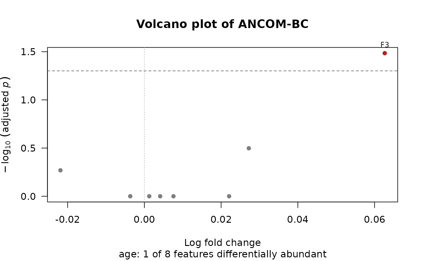
#> 12 F3 age 0.0626 0.0218 2.87 0.00409 0.0328 TRUE
#> # Attributes: method, formula, alpha, p_adjust, log_base, max_iters, tol,
#> # pseudocount, coef, var, vcov, design, bias, n_iters, resid_sd, mean
# A volcano plot of one covariate, here the first: moderate vs mild.
plot(res)
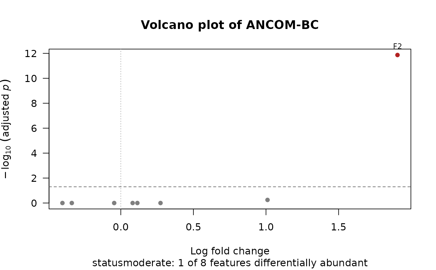 plot(res, 'age')
 # ANCOM-BC2, with zeros as missing values, and (by default) the
# sensitivity analysis: only decisions that hold at pseudocounts 0.1,
# 0.5 and 1 too are kept in `reject_robust`.
res2 <- ancombc2(x, ~ status + age, meta, groups = 'status')
res2[res2$reject, ]
#> # A data.frame: 0 × 10
#> # ANCOM-BC2
#> feature covariate log_fc se w p_value p_adjusted reject passed_ss
#> <chr> <chr> <dbl> <dbl> <dbl> <dbl> <dbl> <lgl> <lgl>
#> # … 1 more column: reject_robust <lgl>
#> # Attributes: method, formula, groups, alpha, p_adjust, log_base, max_iters,
#> # tol, var_quantile, pseudocount, coef, var, vcov, dof, design, bias,
#> # n_iters, resid_sd, mean, sample_fractions, sensitivity
# ANCOMBC's preprocessing, done first: keep features present in at
# least 10% of samples (prv_cut = 0.1), and samples with at least 10
# reads (lib_cut = 10).
x <- x[, colMeans(x > 0) >= 0.1, drop = FALSE]
x <- x[rowSums(x) >= 10, , drop = FALSE]