
Compositional Analysis of Microbiome Data
Source:vignettes/articles/compositional.Rmd
compositional.RmdWhy sequencing data are compositional
Amplicon (16S, ITS) and shotgun metagenomic sequencing don’t count every microbe in a sample. They count a few thousand to a few million reads drawn from a library of fixed size, and that size is set by the sequencer, not by the biology. A sample’s read total therefore carries no information about how many microbes were there, and each taxon’s count is only meaningful relative to the other taxa in the same sample. Data like this are compositional: they live on a simplex, and only the ratios between parts are informative.
That has practical consequences, explained in the open-access reviews by Gloor et al. (2017) and Quinn et al. (2018):
- When one taxon blooms, every other taxon’s relative abundance falls, even if its absolute abundance didn’t change. Tests on relative abundances then report many false “decreases”.
- Correlations between relative abundances are distorted by the closure and change when taxa are added to or dropped from the table.
- Results depend on the arbitrary choices used to deal with zeros.
The log ratio of two taxa is unaffected by all of this: it is the same whether you compute it from absolute abundances, relative abundances or raw read counts. Compositional data analysis (CoDa; Aitchison 1982) builds every method on log ratios.
This article walks through a compositional workflow with ecodive. Most of the functions are already in ecodive; the rest are planned. For each planned function the article shows the call it will have, marked planned, followed by an established package that does the job today.
| Step | Question | In ecodive now | Planned |
|---|---|---|---|
| Zeros | How do I take logs of zeros? |
pseudocount, norm = 'rclr',
replace_zeros() ('mult') |
Bayesian-multiplicative methods ('gbm',
…) |
| Transforms | Which log-ratio coordinates? |
normalize(norm = 'clr' / 'rclr'),
alr(), ilr(), philr()
|
|
| Beta diversity | Do communities differ? |
aitchison(),
robust_aitchison(), rpca(),
rpca_phylo(), pca(), permanova(),
permdisp(), philr_distance()
|
|
| Log ratios | Which taxa shift relative to which? |
rpca() loadings, log_ratio(),
balance()
|
|
| Differential abundance | Which taxa differ? |
ancom(), dirmult_ttest(),
ancombc(), ancombc2() and their post-hoc
tests, structural_zeros()
|
|
| Co-occurrence | Which taxa move together? |
vlr(), rho_p(),
phi_s()
|
|
| Absolute abundance | Did taxa really increase? |
qmp_scale(),
qmp_rarefy()
|
|
| Repeated measures and multi-omics | Subjects over time; several ’omics |
ctf(), rpca_joint()
|
A simulated study
Simulated data let us compare every method with the truth. Forty stool samples, 20 controls and 20 treated, contain 150 taxa (ASVs). In the treated group the five most abundant taxa bloom 8-fold and taxa 6–10 drop 4-fold, in absolute terms; the other 140 taxa don’t change. Each sample is then “sequenced”: its composition is sampled at a random depth of 5,000–40,000 reads, as a sequencer would.
library(ecodive)

set.seed(42)
n_taxa <- 150
groups <- rep(c('control', 'treated'), each = 20)
n      <- length(groups)
taxa   <- sprintf('ASV%03d', seq_len(n_taxa))
samples <- sprintf('S%02d', seq_len(n))

# Typical absolute abundance of each taxon: heavy-tailed, sorted so that
# ASV001 is the most abundant.
base <- sort(exp(rnorm(n_taxa, mean = 0, sd = 2)), decreasing = TRUE)

# True fold changes in absolute abundance (treated vs control).
fold <- rep(1, n_taxa)
fold[1:5]  <- 8      # blooms
fold[6:10] <- 1 / 4  # declines
changed    <- fold != 1

# Absolute abundances: the group effect, plus biological noise, plus
# patchy absences of the rarer taxa.
absolute <- t(sapply(groups, function (g) {
  mu <- if (g == 'treated') base * fold else base
  mu * exp(rnorm(n_taxa, 0, 0.5)) }))
patchy <- matrix(runif(n * n_taxa) < 0.3, n, n_taxa)
patchy[, 1:20] <- FALSE
absolute[patchy] <- 0
dimnames(absolute) <- list(samples, taxa)

# Total microbial load (e.g. cells per gram), which in a real study would
# have to be measured separately.
load <- rowSums(absolute)

# Sequencing: draw reads from each sample's composition.
depth  <- round(runif(n, 5000, 40000))
counts <- t(sapply(seq_len(n), function (i) rmultinom(1, depth[i], absolute[i, ])))
dimnames(counts) <- list(samples, taxa)

counts[1:5, 1:6]
#>     ASV001 ASV002 ASV003 ASV004 ASV005 ASV006
#> S01   8584   1695   4009   1480   1236    461
#> S02   7078   4514   1776   1924   1166    705
#> S03   3198   2471   1677   1102   1150    571
#> S04   6436   3919   3026   2170    959   1674
#> S05   4966   1842   2315   2375    618   1273
mean(counts == 0)  # proportion of zeros
#> [1] 0.3563333

# Taxa found in at least 90% of samples, for the steps that need them.
prevalent <- colMeans(counts > 0) >= 0.9
sum(prevalent)
#> [1] 20
The problem, in one test
Compare each unchanged taxon between groups with a Wilcoxon test, first on the true absolute abundances, then on relative abundances (the usual approach):
rel <- counts / rowSums(counts)

wilcox_p <- function (x) wilcox.test(x ~ groups, exact = FALSE)$p.value

p_abs <- apply(absolute[, !changed], 2, wilcox_p)
p_rel <- apply(rel[, !changed], 2, wilcox_p)

# Proportion of the 140 unchanged taxa called "different" at p < 0.05
c(absolute = mean(p_abs < 0.05), relative = mean(p_rel < 0.05))
#>   absolute   relative
#> 0.08571429 0.63571429
The bloom of five taxa pushes every other taxon’s share down, so most taxa that didn’t change look as if they decreased. A log ratio between two unchanged taxa doesn’t have this problem, because both shares fall by the same factor:
pair <- c('ASV011', 'ASV012')                  # two unchanged taxa
true_prop <- absolute / rowSums(absolute)      # true relative abundances

lr_abs  <- log(absolute[, pair[1]]  / absolute[, pair[2]])
lr_prop <- log(true_prop[, pair[1]] / true_prop[, pair[2]])
all.equal(lr_abs, lr_prop)   # identical, whatever happened to the total
#> [1] TRUE

# The ratio of read counts estimates the same quantity, up to sampling noise:
lr_counts <- log(counts[, pair[1]] / counts[, pair[2]])
cor(lr_abs, lr_counts)
#> [1] 0.9842692
The rest of this article builds on that idea.
Zeros
About a third of this table is zeros, which is typical of amplicon data. A log of zero is undefined, and how zeros are handled can change results (Gloor et al. 2017; Lubbe et al. 2021). There are three families of approaches.
1. Add a pseudocount (available). Every function
with norm = 'clr' takes pseudocount, added to
every cell. With the default NULL, ecodive uses half the
smallest non-zero value and warns. Simple, but it changes the ratios
between the non-zero taxa, most for shallow samples.
2. Treat zeros as missing (available). The
robust clr (rclr) uses only the non-zero values of
each sample, leaving zeros out entirely. It underlies
robust_aitchison() and rpca() (Martino et al.
2019), which complete the missing values with a low-rank
model.
3. Replace zeros multiplicatively
(replace_zeros()). Each zero gets a small value, and the
sample’s non-zero parts are shrunk by a common factor, so the ratios
between them are preserved. The Bayesian-multiplicative versions choose
each zero’s value from the data (Martín-Fernández et
al. 2015). The geometric Bayesian-multiplicative method
(GBM) of the zCompositions package (Palarea-Albaladejo
& Martín-Fernández 2015) is the most used in microbiome
work.
ecodive has simple multiplicative replacement (the method of
scikit-bio’s multi_replace()), in which every zero gets the
same small proportion delta:
zf <- replace_zeros(counts, 'mult')   # the same as replace_zeros_mult(counts)
range(rowSums(zf))                    # proportions, with no zeros left
#> [1] 1 1
sum(zf == 0)
#> [1] 0
# Planned in ecodive: the Bayesian-multiplicative methods
zf <- replace_zeros(counts, 'gbm')    # or replace_zeros_gbm(counts)

# Available now, in zCompositions (CRAN):
# (by default it drops taxa or samples that are at least 80% zeros)
zf <- zCompositions::cmultRepl(counts, method = 'GBM', output = 'prop')
A zero-free table needs no pseudocount, so it goes straight into any
function with norm = 'clr', aitchison(),
alr(), ilr(), vlr() and
rho_p().
Check that your conclusions don’t depend on the choice. Here is the same PERMANOVA under three treatments of zeros. The conclusion holds in all three, but the effect size (R²) depends on the choice:
zero_treatments <- list(
  'pseudocount = 1'     = aitchison(counts, pseudocount = 1),
  'multiplicative'      = aitchison(replace_zeros(counts, 'mult')),
  'robust (rclr)'       = robust_aitchison(counts) )

t(sapply(zero_treatments, function (dm) {
  res <- permanova(dm, groups, seed = 1)
  c(R2 = res$r2, F = unname(res$statistic), p = res$p_value) }))
#>                         R2        F     p
#> pseudocount = 1 0.07759500 3.196654 0.001
#> multiplicative  0.08185786 3.387927 0.001
#> robust (rclr)   0.14845324 6.624678 0.001
As more methods join replace_zeros(),
list_zero_replacements() makes this a loop over all of
them.
Used in practice. Schoeler et al. (2023) replaced the zeros in human shotgun metagenomic counts by geometric Bayesian-multiplicative replacement before a clr transform, as did Vervier et al. (2022) for the taxonomic profiles of people with irritable bowel syndrome. Romano et al. (2021) used the count-zero multiplicative variant in a 16S meta-analysis of Parkinson’s disease.
Log-ratio transforms
A transform maps each sample’s composition to real-valued coordinates where ordinary statistics apply.
| Transform | ecodive | Coordinates | Notes |
|---|---|---|---|
| centered log ratio (clr) |
normalize(norm = 'clr'), or
norm = 'clr' in beta_div(),
pca(), envfit(), rda(), … |
one per taxon, relative to the sample’s geometric mean | the most used; its coordinates sum to 0 |
| robust clr (rclr) | normalize(norm = 'rclr') |
non-zero taxa only | zeros are missing, not imputed |
| additive log ratio (alr) | alr() |
each taxon relative to one reference taxon | easy to interpret; not isometric |
| isometric log ratio (ilr) | ilr() |
D − 1 orthonormal balances | Euclidean distance on ilr = Aitchison distance |
| phylogenetic ilr (PhILR) | philr() |
one balance per internal node of a phylogeny | Silverman et al. 2017 |
a <- alr(counts, denominator = 'ASV001', pseudocount = 1)
dim(a)
#> [1]  40 149

# Median group difference of the alr coordinates (treated - control):
median(colMeans(a[groups == 'treated', ]) - colMeans(a[groups == 'control', ]))
#> [1] -1.28805

i <- ilr(counts, pseudocount = 1)   # default (Helmert) basis
dim(i)
#> [1]  40 149

# Euclidean distances between ilr coordinates are Aitchison distances:
all.equal(as.vector(dist(i)), as.vector(aitchison(counts, pseudocount = 1)))
#> [1] TRUE
Here the alr makes the point of the previous section in another way: ASV001 is one of the blooming taxa, so the alr coordinates fall in the treated group whether or not the taxa changed (by log 8 ≈ 2.1 for taxa without zeros; less for rare taxa, where zeros and the pseudocount damp it). An alr reference should be a taxon that is common and stable, which is hard to know in advance.
For prediction, these transforms serve
interpretation and compositional geometry; don’t expect them to make a
machine-learning model more accurate. With random forests predicting 65
metadata variables in four datasets, Yerke et al. (2024)
found that alr, clr and ilr (PhILR) “performed generally slightly worse
or only as well as compositionally naïve transformations”; relative
abundances did best, by a small margin. Compare with relative abundances
(normalize(counts, 'percent')) before choosing a log-ratio
predictor table.
PhILR needs a phylogeny. The simulated taxa get one that puts the five blooming taxa in one clade and the five declining taxa in another, and joins the other 140 at random:
set.seed(7)
random_clade <- function (tips) {
  len <- runif(1, 0.05, 0.3)
  if (length(tips) == 1) return (sprintf('%s:%.3f', tips, len))
  k <- sample(length(tips) - 1, 1)
  sprintf('(%s,%s):%.3f', random_clade(tips[1:k]), random_clade(tips[-(1:k)]), len)
}
tree <- read_tree(sprintf('(%s,(%s,%s):0.2);',
  random_clade(taxa[1:5]), random_clade(taxa[6:10]),
  random_clade(sample(taxa[-(1:10)])) ))
c(tips = length(tree$tip.label), internal_nodes = tree$Nnode)
#>           tips internal_nodes
#>            150            149
philr() gives one balance per internal node of the tree.
These weights are those of Silverman et al. (2017), as in the philr
package (Bioconductor):
p <- philr(counts, tree, pseudocount = 1,
           part_weights = 'enorm.x.gm.counts', ilr_weights = 'blw.sqrt')
dim(p)   # one coordinate per internal node of the 150-tip tree
#> [1]  40 149
Used in practice. Ruuskanen et al. (2021) PhILR-transformed shotgun metagenomes from the FINRISK cohort and modelled the balances to find clades linked to fatty liver; Worsley et al. (2021) used both clr and PhILR coordinates of 16S data from a wild bird population.
Beta diversity and ordination
The Aitchison distance is the Euclidean distance between clr coordinates, and it is the compositional counterpart of Bray-Curtis. Its robust version uses the rclr. Both work with every ecodive ordination and test.
dm_ait  <- aitchison(counts, pseudocount = 1)
dm_rait <- robust_aitchison(counts)

# Do the groups differ in composition, and in dispersion?
permanova(dm_rait, groups, seed = 1)
#> Permutational multivariate analysis of variance (PERMANOVA) of Robust Aitchison Distance
#>
#> F = 6.625, p = 0.001, z = 23.86
#> Permutations: 999 (free)
#>
#> Model R2 = 0.1485. Model tested as a whole:
#>
#>          Df SumOfSqs     R2     F Pr(>F)
#> Model     1      668 0.1485 6.625  0.001 ***
#> Residual 38     3834 0.8515
#> Total    39     4503 1.0000
#> ---
#> Signif. codes:  0 '***' 0.001 '**' 0.01 '*' 0.05 '.' 0.1 ' ' 1
permdisp(dm_rait, groups, seed = 1)
#> Homogeneity of multivariate dispersions (PERMDISP) of Robust Aitchison Distance
#>
#> F =  24.4, p = 0.001, z = 15.19
#> Permutations: 999 (free)
#>
#> Distances to group centroids:
#> control treated
#>  10.313   9.185
#>
#>           Df Sum Sq Mean Sq    F N.Perm Pr(>F)
#> Groups     1  12.72  12.725 24.4    999  0.001 ***
#> Residuals 38  19.82   0.522
#> ---
#> Signif. codes:  0 '***' 0.001 '**' 0.01 '*' 0.05 '.' 0.1 ' ' 1
Both are significant here: the treated samples, dominated by the same
blooming taxa, are also more alike than the controls.
permdisp() matters because PERMANOVA can’t tell a shift in
location from a difference in spread (Anderson & Walsh
2013).
Robust Aitchison PCA (rpca()) ordinates
the rclr table directly, completing the missing (zero) entries with a
low-rank model, and returns taxon loadings for a biplot. It is the
method of DEICODE and of QIIME 2’s gemelli plugin (Martino et al.
2019).
ord <- rpca(counts, n_axes = 2)
ord   # its title, % of variance per axis, and first samples
#> # A matrix: 40 samples × 2 axes
#> # Robust Aitchison PCA
#> # % of variance: 93.1, 6.9
#>     RPCA1   RPCA2
#> S01 -4.47  0.513
#> S02 -4.67  0.21
#> S03 -5.12  0.788
#> S04 -2.55 -0.31
#> S05 -6.01  0.889
#> S06 -4.19  0.0524
#> S07 -4.84  0.369
#> S08 -4.89  0.302
#> S09 -3.71  0.245
#> S10 -5.01  1.15
#> # … 30 more samples
#> # Use print(x, n = ...) to see more samples
#> # Attributes: method, eig, prop, trace, loadings, cost, n_iters

# A biplot: the samples by group, and the ten longest taxon loadings.
grp <- groups[match(rownames(ord), rownames(counts))]
plot(ord, grp, col = c('#4E9FDE', '#E8854A'))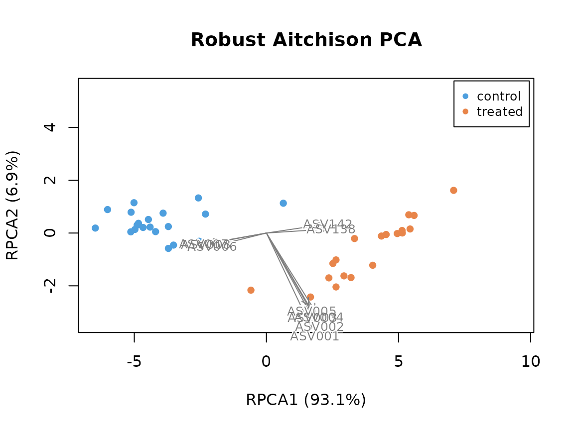
A clr PCA (pca(counts, norm = 'clr', pseudocount = 1))
or a PCoA of the Aitchison distances (pcoa(dm_ait)) gives
the classic “Aitchison PCA” with a pseudocount instead.
Phylogenetic RPCA (rpca_phylo();
Martino et
al. 2022) runs RPCA on counts summed over every clade of a
phylogeny, weighted by branch length, so clades that shift together show
up as single features. It’s the compositional counterpart of a UniFrac
PCoA, and gives loadings for every clade as well as every tip.
It uses the tree built for PhILR above. As
in the log ratios below, rare tips get large
loadings from noise alone, so leave out tips present in half the samples
or fewer (min_feature_frequency, a percentage, as in
rpca()):
ord_phy <- rpca_phylo(counts, tree, n_axes = 2, min_feature_frequency = 50)
ord_phy
#> # A matrix: 40 samples × 2 axes
#> # Phylogenetic Robust Aitchison PCA
#> # % of variance: 94.7, 5.3
#>     RPCA1   RPCA2
#> S01 -5.17  0.273
#> S02 -4.52  0.719
#> S03 -5.8  -0.254
#> S04 -3.58 -0.482
#> S05 -5.01  0.954
#> S06 -2.96  0.853
#> S07 -4.92  0.0509
#> S08 -4.33  0.295
#> S09 -2.49  1.29
#> S10 -4.77  0.0854
#> # … 30 more samples
#> # Use print(x, n = ...) to see more samples
#> # Attributes: method, eig, prop, trace, loadings, cost, n_iters, tree

# The nodes with the largest loadings on the first axis:
load_phy <- attr(ord_phy, 'loadings')[, 1]
round(head(load_phy[order(-abs(load_phy))], 6), 3)
#>   n232 ASV002     n2     n6 ASV004     n7
#>  0.226  0.223  0.220  0.219  0.215  0.215

# Internal nodes are named "n<id>"; this lists the tips below one.
tips_below <- function (tree, node) {
  ntip <- length(tree$tip.label)
  ids  <- ntip + match(node, tree$node.label)
  repeat {
    more <- union(ids, tree$edge[tree$edge[, 1] %in% ids, 2])
    if (length(more) == length(ids)) break
    ids <- more
  }
  sort(tree$tip.label[ids[ids <= ntip]])
}
top_node <- names(load_phy)[which.max(abs(load_phy))]
tips_below(attr(ord_phy, 'tree'), top_node)
#> [1] "ASV001" "ASV002" "ASV003" "ASV004" "ASV005"
The top node is the clade of the five blooming taxa.
attr(ord_phy, 'tree') is the tree as it was used (pruned to
the kept tips), with its internal nodes named as in the loadings.
The PhILR distance is the Euclidean distance between PhILR coordinates, with the weights of Silverman et al. (2017):
# The same as beta_div(counts, 'philr', tree = tree, pseudocount = 1):
dm_philr <- philr_distance(counts, tree, pseudocount = 1)
permanova(dm_philr, groups, seed = 1)
#> Permutational multivariate analysis of variance (PERMANOVA) of PhILR Distance
#>
#> F = 32.33, p = 0.001, z = 43.02
#> Permutations: 999 (free)
#>
#> Model R2 = 0.4597. Model tested as a whole:
#>
#>          Df SumOfSqs     R2     F Pr(>F)
#> Model     1    14210 0.4597 32.33  0.001 ***
#> Residual 38    16702 0.5403
#> Total    39    30912 1.0000
#> ---
#> Signif. codes:  0 '***' 0.001 '**' 0.01 '*' 0.05 '.' 0.1 ' ' 1
Rarefied or compositional? Rarefying every sample to
the same depth is the other answer to uneven sequencing depth, and
Schloss (2024,
2026)
argues that it controls for depth better than robust Aitchison PCA does:
correcting “numerous problems” in the benchmark that had supported
robust Aitchison PCA, he found that it “was not insensitive to uneven
sequencing effort and did not perform as well as rarefaction”. So
rpca() is not a correction for depth (its help explains
why, under “Sequencing depth”). Averaging many rarefactions
(beta_div_rarefied()) removes most of the noise that a
single one adds. A Procrustes test shows how far the two views agree on
these samples, and envfit() whether either ordination still
follows sequencing depth:
dm_rare  <- beta_div_rarefied(counts, 'bray', times = 20)
dm_rare
#> # A dist: 40 samples (lower triangle)
#> # Bray-Curtis Dissimilarity (rarefied 20×)
#>       S01   S02   S03   S04   S05   S06   S07   S08   S09   S10
#> S02 0.244
#> S03 0.367 0.298
#> S04 0.275 0.227 0.32
#> S05 0.306 0.305 0.296 0.272
#> S06 0.278 0.281 0.371 0.33  0.384
#> S07 0.251 0.178 0.302 0.238 0.279 0.287
#> S08 0.329 0.272 0.265 0.237 0.256 0.33  0.255
#> S09 0.24  0.235 0.271 0.204 0.313 0.259 0.217 0.219
#> S10 0.33  0.276 0.265 0.259 0.264 0.346 0.257 0.242 0.259
#> S11 0.281 0.278 0.315 0.314 0.322 0.305 0.285 0.333 0.268 0.323
#> # … 29 more samples
#> # Use print(x, n = ...) to see more samples
#> # Attributes: method, depth, dropped
ord_rare <- pcoa(dm_rare, n_axes = 2)
procrustes_test(ord_rare, ord, seed = 1)
#> Procrustes randomization test (PROTEST)
#>
#> r = 0.7434, p = 0.001, z =     8
#> Permutations: 999 (free)
#>
#> Symmetric Procrustes sum of squares (m^2): 0.4474
#> Samples: 40, axes: 2

log_depth <- data.frame(log_depth = log(rowSums(counts)))
envfit(ord_rare, log_depth, seed = 1)
#> # A data.frame: 1 × 7
#> # Fitted variables on Principal Coordinates Analysis of Bray-Curtis Dissimilarity (rarefied 20×)
#>           variable  level   PCoA1 PCoA2     r2 p_value     z
#>           <chr>     <chr>   <dbl> <dbl>  <dbl>   <dbl> <dbl>
#> log_depth log_depth NA    0.00208    -1 0.0806   0.209 0.616
#> # Attributes: r2_perm, n_perm
envfit(ord, log_depth, seed = 1)
#> # A data.frame: 1 × 7
#> # Fitted variables on Robust Aitchison PCA
#>           variable  level  RPCA1  RPCA2    r2 p_value     z
#>           <chr>     <chr>  <dbl>  <dbl> <dbl>   <dbl> <dbl>
#> log_depth log_depth NA    -0.166 -0.986 0.499   0.001  8.75
#> # Attributes: r2_perm, n_perm
The larger an ordination’s r² for log_depth, the more it
still reflects how deeply each sample happened to be sequenced rather
than what is in it.
Is it depth? The comparison above changes two things at once, the metric and the rarefying. Two more checks separate them: the correlation of each RPCA axis with log library size, and PCoAs of the robust Aitchison distance (the same rclr, without RPCA’s completion of the zeros), as it is and averaged over rarefactions:
# Correlation of each RPCA axis with log library size:
cor(ord, log_depth[rownames(ord), , drop = FALSE])
#>        log_depth
#> RPCA1 -0.3721507
#> RPCA2 -0.6002383

ord_rait  <- pcoa(dm_rait, n_axes = 2)
ord_rrare <- pcoa(beta_div_rarefied(counts, 'robust_aitchison', times = 20), n_axes = 2)
envfit(ord_rait, log_depth, seed = 1)
#> # A data.frame: 1 × 7
#> # Fitted variables on Principal Coordinates Analysis of Robust Aitchison Distance
#>           variable  level  PCoA1  PCoA2    r2 p_value     z
#>           <chr>     <chr>  <dbl>  <dbl> <dbl>   <dbl> <dbl>
#> log_depth log_depth NA    -0.874 -0.486 0.167   0.038  2.35
#> # Attributes: r2_perm, n_perm
envfit(ord_rrare, log_depth, seed = 1)
#> # A data.frame: 1 × 7
#> # Fitted variables on Principal Coordinates Analysis of Robust Aitchison Distance (rarefied 20×)
#>           variable  level  PCoA1  PCoA2     r2 p_value     z
#>           <chr>     <chr>  <dbl>  <dbl>  <dbl>   <dbl> <dbl>
#> log_depth log_depth NA    -0.118 -0.993 0.0934   0.142 0.963
#> # Attributes: r2_perm, n_perm
procrustes_test(ord_rrare, ord, seed = 1)
#> Procrustes randomization test (PROTEST)
#>
#> r = 0.8299, p = 0.001, z = 8.734
#> Permutations: 999 (free)
#>
#> Symmetric Procrustes sum of squares (m^2): 0.3113
#> Samples: 40, axes: 2
The RPCA follows depth most: its second axis correlates −0.60 with
log library size, and envfit() gave it r² = 0.50 (p =
0.001). The robust Aitchison PCoA follows it less (r² = 0.17, p =
0.038), and the rarefied one least (r² = 0.09, p = 0.14, close to the
rarefied Bray-Curtis PCoA’s 0.08), while still agreeing well with the
RPCA (Procrustes r = 0.83, against 0.74 for Bray-Curtis). On these
simulated samples, then, most of RPCA’s depth signal comes with the
completion of the zeros, and rarefying lowers what is left. That is one
simulation, not a benchmark: run the same checks on your own data.
Used in practice.
- Aitchison distance and clr PCA: Bian et al. (2017), a 16S study of healthy people aged 3 to over 100; Romano et al. (2021), with PERMANOVA on Aitchison distances.
- Robust Aitchison PCA (DEICODE): Dong et al. (2022), obesity and the brain-gut axis; Bermudez-Martin et al. (2021), a mouse study, on non-rarefied tables.
- Phylogenetic RPCA: Dokoshi et al. (2024), skin injury and the gut microbiome in mice; DeClercq et al. (2025), the salivary microbiome in inflammatory bowel disease, alongside Aitchison, robust Aitchison, Bray-Curtis and UniFrac distances.
Log ratios and balances
Log ratios between groups of taxa are what can be interpreted without assumptions about total load (Morton et al. 2019). A common recipe is to take the taxa at the two ends of an RPCA axis (or of a model’s ranked coefficients), and analyse the log ratio of the top ones over the bottom ones as a single per-sample variable. Qurro does this interactively (Fedarko et al. 2020). Choose among prevalent taxa: rare taxa can have large loadings from noise alone, and their sums are often zero.
load_ax1 <- attr(ord, 'loadings')[, 1]
load_ax1 <- load_ax1[names(load_ax1) %in% taxa[prevalent]]
top    <- names(sort(load_ax1, decreasing = TRUE))[1:5]
bottom <- names(sort(load_ax1))[1:5]
top
#> [1] "ASV002" "ASV004" "ASV001" "ASV003" "ASV005"
bottom
#> [1] "ASV007" "ASV008" "ASV006" "ASV009" "ASV010"
log_ratio() gives one value per sample, which can go
straight into any test or model, or into the metadata:
lr <- log_ratio(counts, numerator = top, denominator = bottom)   # log of summed counts
tapply(lr, groups, median)
#>  control  treated
#> 1.424839 4.852423
wilcox.test(as.vector(lr) ~ groups, exact = FALSE)$p.value
#> [1] 6.795615e-08
Which way the axis points depends on its sign, so check which group
the “top” taxa belong to before interpreting (here, compare with the
true fold):
A balance (balance()) uses geometric
means instead of sums, scaled so that balances of different sizes are
comparable; it is one coordinate of an ilr().
b <- balance(counts, numerator = top, denominator = bottom, pseudocount = 1)
tapply(b, groups, median)
#>  control  treated
#> 1.984592 7.407924
selbal searches for the balance that best predicts an outcome (Rivera-Pinto et al. 2018). coda4microbiome does the same for cross-sectional and longitudinal studies (Calle et al. 2023).
Used in practice. Taylor et al. (2020) ranked taxa by their association with eating fermented plants (Songbird), then compared the log ratio of the top- over the bottom-ranked taxa between consumers and non-consumers in Qurro. Xue et al. (2025) reported an Akkermansiaceae / Muribaculaceae log ratio in a mouse model of sleep apnoea. Trøseid et al. (2023) built a dysbiosis index for severe COVID-19 as a selbal balance and related it to 60-day mortality.
Differential abundance
Per-taxon tests need a reference that the compositional effect cancels against, and methods differ in how they choose it. Different methods give different answers on the same data (Nearing et al. 2022), so report results that agree across two or more of them.
| Method | Reference | ecodive | Elsewhere |
|---|---|---|---|
| ANCOM | every other taxon: tests all pairwise log ratios | ancom() |
scikit-bio, QIIME 2 |
| ALDEx2-style | clr of Dirichlet Monte Carlo draws | dirmult_ttest() |
ALDEx2 (Bioconductor), scikit-bio |
| ANCOM-BC / ANCOM-BC2 | estimates the shift shared by all taxa as a bias, and removes it |
ancombc(), ancombc2()
|
ANCOMBC (Bioconductor), scikit-bio |
ANCOM (Mandal et al. 2015) counts, for each taxon, how many of its log ratios with other taxa differ between groups (its W), and declares the taxa with the largest W differentially abundant:
res_ancom <- ancom(counts, groups, pseudocount = 1)
res_ancom[order(-res_ancom$W), ]
#> # A data.frame: 150 × 3
#> # ANCOM: control vs treated
#>    feature     W reject
#>    <chr>   <int>  <lgl>
#> 8  ASV008    131   TRUE
#> 7  ASV007    120   TRUE
#> 9  ASV009    111  FALSE
#> 6  ASV006    110  FALSE
#> 10 ASV010    110  FALSE
#> 4  ASV004     85  FALSE
#> 2  ASV002     79  FALSE
#> 3  ASV003     58  FALSE
#> 1  ASV001     54  FALSE
#> 5  ASV005     51  FALSE
#> # … 140 more rows
#> # Use print(x, n = ...) to see more rows
#> # Attributes: method, groups, sig_test, p_adjust, alpha, tau, theta, cutoff,
#> #   pseudocount
table(changed = changed, rejected = res_ancom$reject)
#>        rejected
#> changed FALSE TRUE
#>   FALSE   140    0
#>   TRUE      8    2
plot(res_ancom)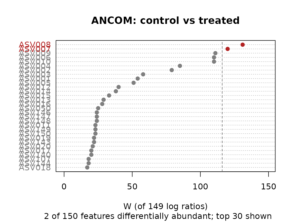
W ranks the ten changed taxa first, but ANCOM’s cutoff rule declares only two of them: it is conservative, and gives no effect sizes.
ALDEx2
(Fernandes et al. 2014) carries the uncertainty of low counts through
Monte Carlo draws from a Dirichlet distribution, takes the clr of each
draw, and tests each taxon. dirmult_ttest() is scikit-bio’s
version, with Welch’s t-test; contrast is
c(treatment, reference):
res_dm <- dirmult_ttest(counts, groups, contrast = c('treated', 'control'))
res_dm[order(res_dm$p_adjusted), ]
#> # A data.frame: 150 × 11
#> # Dirichlet-multinomial t-test
#>    feature      t log2_fc ci_lower ci_upper pooled_sd  mean effect  p_value
#>    <chr>    <dbl>   <dbl>    <dbl>    <dbl>     <dbl> <dbl>  <dbl>    <dbl>
#> 4  ASV004   12.1     2.52     1.96     3.06     0.66   8.68   3.83 3.51e-14
#> 2  ASV002   10.6     2.45     1.81     3.04     0.73   9.59   3.36 2.31e-12
#> 8  ASV008  -11.2    -3.11    -4.01    -2.31     0.885  5.02  -3.54 1.12e-11
#> 3  ASV003    9.9     2.28     1.66     2.85     0.729  8.92   3.13 3.37e-11
#> 1  ASV001    8.79    2.22     1.55     2.86     0.801 10.7    2.78 1.92e-10
#> 10 ASV010   -9.25   -2.51    -3.32    -1.73     0.86   4.7   -2.93 5.73e-10
#> 9  ASV009   -8.56   -2.57    -3.49    -1.72     0.953  4.97  -2.71 5.94e-10
#> 5  ASV005    8.29    2.21     1.49     2.88     0.844  8.29   2.62 2.11e-09
#> 7  ASV007   -9      -2.94    -4.02    -2.03     1.04   5.02  -2.85 2.81e-09
#> 6  ASV006   -8.44   -2.67    -3.75    -1.83     1.01   5.01  -2.67 7.14e-09
#> # … 140 more rows
#> # … 2 more columns: p_adjusted <dbl>, reject <lgl>
#> # Use print(x, n = ...) to see more rows
#> # Attributes: method, contrast, n, n_draws, pseudocount, scale_sd, alpha,
#> #   conf_level, p_adjust, seed, log_base
table(changed = changed, rejected = res_dm$reject)
#>        rejected
#> changed FALSE TRUE
#>   FALSE   140    0
#>   TRUE      0   10
plot(res_dm)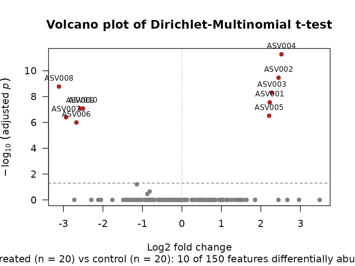
It finds all ten changed taxa and nothing else. But compare its fold changes with the truth, log2(8) = 3 for the blooms and log2(1/4) = −2 for the declines:
tapply(res_dm$log2_fc[changed], fold[changed], median)
#>      0.25         8
#> -2.672671  2.277540
Every estimate is shifted down by about 0.7 log2 units, which is the subject of the next section.
A volcano plot can mislead: with many samples, tiny differences reach small p-values (Gloor, Macklaim & Fernandes 2016). The effect plot (ALDEx2’s “MW” plot) sets each taxon’s difference between the groups against its spread within them; taxa beyond the dashed lines differ by more than they vary:
plot(res_dm, 'effect')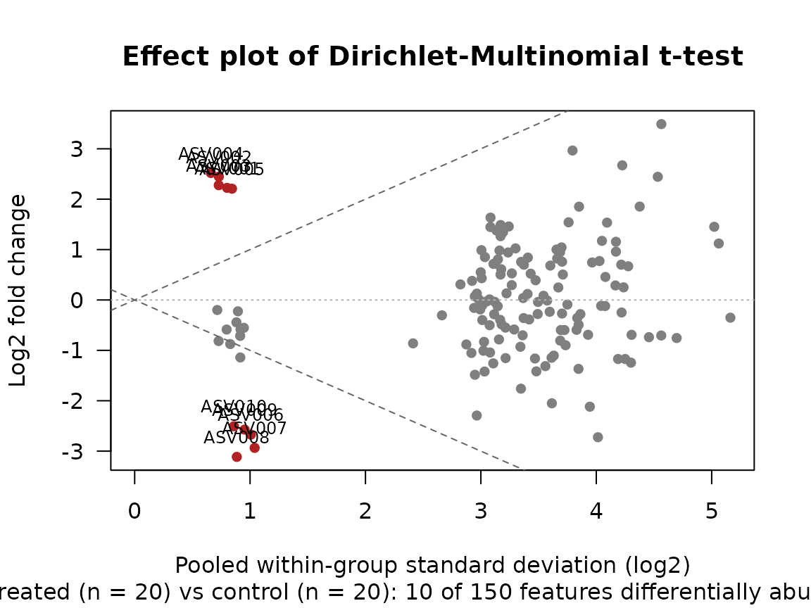
type = 'ma' plots the differences against each taxon’s
mean abundance, and type = 'forest' the most significant
taxa with their intervals; the same types work for
ancombc(), ancombc2(), da_ttest()
and da_lm().
Why the reference matters
Every per-taxon method compares each taxon with some reference. With relative abundances the reference is the sample’s total, which the bloom inflates; with the clr it is the sample’s geometric mean over all taxa. Compare the estimated group difference (natural log) for the prevalent unchanged taxa, whose true difference is 0:
ok <- !changed & prevalent
d_rel <- colMeans(log(rel[groups == 'treated', ok])) -
         colMeans(log(rel[groups == 'control', ok]))
d_clr <- colMeans(clr[groups == 'treated', ok]) -
         colMeans(clr[groups == 'control', ok])
rbind(relative = summary(d_rel), clr = summary(d_clr))
#>                Min.    1st Qu.     Median      Mean    3rd Qu.       Max.
#> relative -1.8256646 -1.5810305 -1.4430368 -1.458607 -1.3557451 -1.1708031
#> clr      -0.9806151 -0.7381877 -0.5979246 -0.614149 -0.5102008 -0.3338742

mean(log(fold))   # the true change in the geometric mean of all 150 taxa
#> [1] 0.02310491
The total is dominated by the five blooming taxa, so relative abundances shift every unchanged taxon down, by about 1.4 on the log scale (an apparent 4-fold decrease). The clr does better, but is still biased, although the true geometric mean hardly changed (only 10 of 150 taxa changed, and partly cancel). The rest of the bias comes from the zeros: in the treated samples the bloom takes reads away from the rare taxa, which get more zeros, and a pseudocount (or any replaced value) doesn’t fall with them, so the estimated geometric mean falls by less than the abundant taxa do.
So a clr-based test rests on two things: an assumption that most taxa
don’t change (or that changes balance out), and the zero treatment. When
either fails, it reports which taxa moved relative to the
average taxon, not in absolute terms. That is the shift seen in
dirmult_ttest()’s fold changes above. ANCOM-BC estimates
the shift as a bias and removes it (next section); measuring total load
removes it outright (see Absolute
abundance); and scale models (Nixon, Gloor &
Silverman 2025) make it uncertain instead of assuming it is
zero. In dirmult_ttest(), scale_sd is the
standard deviation, in log2 units, of a random shift in the typical
taxon’s abundance between the groups, drawn afresh in every Monte Carlo
draw. Nixon et al. suggest 0.5; use more draws with it:
res_sm <- lapply(c(0, 0.5, 1), function (sd)
  dirmult_ttest(counts, groups, contrast = c('treated', 'control'),
                scale_sd = sd, n_draws = 1000) )

data.frame(
  scale_sd       = c(0, 0.5, 1),
  rejected       = sapply(res_sm, function (r) sum(r$reject)),
  false_positive = sapply(res_sm, function (r) sum(r$reject & !changed)),
  ci_width       = sapply(res_sm, function (r) median((r$ci_upper - r$ci_lower)[changed])) )
#>   scale_sd rejected false_positive ci_width
#> 1      0.0       10              0 1.649865
#> 2      0.5       10              0 4.241770
#> 3      1.0        0              0 7.299840
The intervals widen as scale_sd grows, so a taxon is
only declared changed when its change is clear of plausible shifts in
the reference. At 0.5 all ten true changes survive; at 1, a shift of 2
log2 units is plausible, and none does. Choose scale_sd
from what you know about how much total load could differ between your
groups, and report how the rejections change over a range of values, as
above.
Wrong scale assumptions are costly. Over 11 RNA-seq and other sequencing datasets, Dos Santos et al. (2026) found that misspecified scale broke false-discovery control in several common tools, and that a scale model reduced the unacceptably high false discovery rates at a cost in sensitivity: no tool offered both. In differential set analysis (enrichment of groups of taxa or genes), McGovern et al. (2023) found positive predictive values as low as 9% under small errors in the assumed scale.
Removing the shift: ANCOM-BC
ANCOM-BC
(ancombc(); Lin & Peddada 2020) and ANCOM-BC2
(ancombc2(); Lin & Peddada 2024) fit a linear model of
each taxon’s log abundance, with any covariates in a formula, and
estimate the shift shared by all taxa as a bias, from the taxa that
don’t change, then subtract it. ANCOM-BC2 also treats zeros as missing
values rather than adding a pseudocount, and regularises the variances
of rare taxa.
As in the R package (its prv_cut), first drop rare taxa:
they are too sparse to estimate well, and here they are the source of
every false positive (without the filter, ANCOM-BC2 calls 7 of
them).
keep <- colMeans(counts > 0) >= 0.7   # taxa in at least 70% of samples
meta <- data.frame(group = groups, row.names = samples)

fit <- ancombc2(counts[, keep], ~ group, meta)
res_bc <- fit[fit$covariate == 'grouptreated', ]
res_bc[order(res_bc$p_adjusted), ]
#> # A data.frame: 58 × 10
#> # ANCOM-BC2
#>    feature covariate    log_fc    se     w  p_value p_adjusted reject passed_ss
#>    <chr>   <chr>         <dbl> <dbl> <dbl>    <dbl>      <dbl>  <lgl>     <lgl>
#> 8  ASV004  grouptreated   2.23 0.216 10.3  1.48e-12   8.57e-11   TRUE      TRUE
#> 6  ASV003  grouptreated   2.06 0.217  9.49 1.44e-11   8.19e-10   TRUE      TRUE
#> 4  ASV002  grouptreated   2.18 0.231  9.43 1.72e-11   9.65e-10   TRUE      TRUE
#> 10 ASV005  grouptreated   2.01 0.23   8.74 1.24e-10    6.8e-09   TRUE      TRUE
#> 2  ASV001  grouptreated   2.02 0.239  8.47 2.76e-10   1.49e-08   TRUE      TRUE
#> 16 ASV008  grouptreated  -1.68 0.259 -6.51 1.13e-07   6.01e-06   TRUE      TRUE
#> 14 ASV007  grouptreated  -1.56 0.256 -6.09 4.31e-07   2.24e-05   TRUE      TRUE
#> 18 ASV009  grouptreated  -1.3  0.242 -5.37 4.14e-06   0.000211   TRUE      TRUE
#> 12 ASV006  grouptreated  -1.37 0.257 -5.32 4.86e-06   0.000243   TRUE      TRUE
#> 20 ASV010  grouptreated  -1.26 0.25  -5.03 1.22e-05   0.000597   TRUE      TRUE
#> # … 48 more rows
#> # … 1 more column: reject_robust <lgl>
#> # Use print(x, n = ...) to see more rows
#> # Attributes: method, formula, alpha, p_adjust, log_base, max_iters, tol,
#> #   var_quantile, pseudocount, coef, var, vcov, dof, design, bias, n_iters,
#> #   resid_sd, mean, sample_fractions, sensitivity
table(changed = changed[keep], rejected = res_bc$reject)
#>        rejected
#> changed FALSE TRUE
#>   FALSE    48    0
#>   TRUE      0   10

# Estimated log fold changes of the changed taxa, against the truth
# (natural logs: log(1/4) = -1.39, log(8) = 2.08):
tapply(res_bc$log_fc[changed[keep]], fold[keep][changed[keep]], median)
#>      0.25         8
#> -1.367935  2.058516

plot(fit)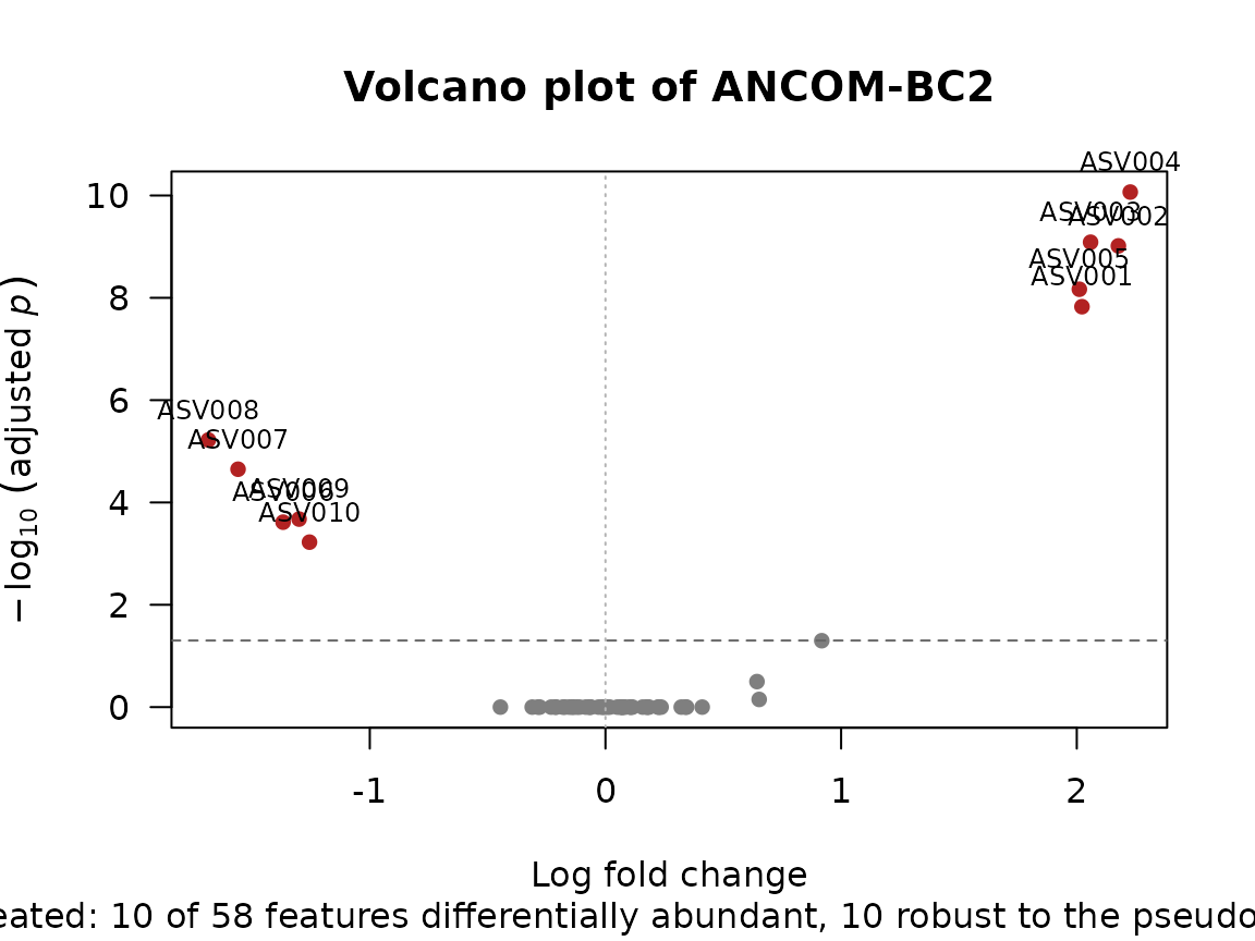
The bias correction recovers the true fold changes almost exactly,
where the clr-based estimates above were off by the shift.
ancombc2() also runs the R package’s sensitivity analysis
by default: it refits with pseudocounts 0.1, 0.5 and 1, and
reject_robust keeps only the decisions that hold in every
fit, which are the ones to report. ANCOM-BC (ancombc())
does a little less well on this table, with two false positives and
estimates further from the truth. It needs a pseudocount for the zeros,
and the bias a pseudocount introduces differs between rare and abundant
taxa, so a single shift can’t remove it all:
fit1 <- ancombc(counts[, keep], ~ group, meta, pseudocount = 1)
res1 <- fit1[fit1$covariate == 'grouptreated', ]
table(changed = changed[keep], rejected = res1$reject)
#>        rejected
#> changed FALSE TRUE
#>   FALSE    46    2
#>   TRUE      0   10
tapply(res1$log_fc[changed[keep]], fold[keep][changed[keep]], median)
#>      0.25         8
#> -1.471240  1.895599
Structural zeros. A taxon absent from every sample
of a group has no log fold change to estimate.
structural_zeros() finds such taxa, so they can be reported
as present in one group only:
sz <- structural_zeros(counts, groups)
sz[rowSums(sz) > 0, , drop = FALSE]
#>        control treated
#> ASV147   FALSE    TRUE
#> ASV150   FALSE    TRUE
Here two rare taxa were never seen in a treated sample.
More than two groups. With a factor of three or more
levels in the formula, name it as groups and run the
post-hoc tests on the fit: ancombc_global() (does the taxon
differ between any groups?), ancombc_pairwise() (every pair
of levels), ancombc_dunnett() (each level against the
reference) and ancombc_trend() (a monotone trend across
ordered levels). Each has a plot() method.
fit3 <- ancombc2(counts, ~ diet + age, meta3, groups = 'diet')
ancombc_global(fit3)
plot(ancombc_pairwise(fit3))
Used in practice. Wallen et al. (2022) counted a species as associated with Parkinson’s disease only when both ANCOM-BC and MaAsLin2 agreed, in shotgun metagenomes from 724 people. Trøseid et al. (2023) used ANCOM-BC2 in severe COVID-19. Mueller et al. (2021) tested metformin’s effect on gut taxa in a randomized trial with ALDEx2.
Co-occurrence: proportionality
Correlations between relative abundances are unreliable (Lovell et al. 2015). Proportionality asks instead whether two taxa keep a constant ratio across samples, using the variance of their log ratio (vlr). The ρp coefficient (Erb & Notredame 2016) rescales it to a correlation-like range, and is the default of the propr package (Quinn et al. 2017).
ecodive’s vlr(), rho_p() and
phi_s() compute every pair of taxa in parallel C, and
return a dist object over the taxa (here on the zero-free
table from the Zeros section):
rho <- rho_p(zf)
length(rho)   # one value for each pair of the 150 taxa
#> [1] 11175

# A dist object puts 0 on the diagonal; rho is 1 there.
m <- as.matrix(rho)
diag(m) <- 1

# Taxa 1-5 bloom together, and 6-10 decline together: each set is
# proportional within itself, and the two sets are anti-proportional.
round(m[1:7, 1:7], 2)
#>        ASV001 ASV002 ASV003 ASV004 ASV005 ASV006 ASV007
#> ASV001   1.00   0.61   0.70   0.69   0.83  -0.77  -0.71
#> ASV002   0.61   1.00   0.72   0.76   0.69  -0.68  -0.79
#> ASV003   0.70   0.72   1.00   0.77   0.71  -0.67  -0.73
#> ASV004   0.69   0.76   0.77   1.00   0.69  -0.72  -0.73
#> ASV005   0.83   0.69   0.71   0.69   1.00  -0.70  -0.69
#> ASV006  -0.77  -0.68  -0.67  -0.72  -0.70   1.00   0.75
#> ASV007  -0.71  -0.79  -0.73  -0.73  -0.69   0.75   1.00
vlr() and phi_s() are dissimilarities, so
they can go straight into pcoa() or hclust()
to ordinate or cluster the taxa. ρp is a similarity: threshold it
(e.g. m > 0.7) to build a network, or use
1 - rho as a dissimilarity.
Used in practice. Auladell et al. (2022) used ρ (propr, at 5% FDR) to ask whether closely related marine bacteria co-vary through the seasons; Chaudhari et al. (2021) built a ρ network of genome-resolved groundwater bacteria from metagenomic coverages.
Absolute abundance
Compositional methods recover ratios, never totals. If you
measure each sample’s total microbial load (flow
cytometry, total 16S qPCR, or a spike-in), you can estimate absolute
abundances instead: quantitative microbiome profiling
(QMP; Vandeputte
et al. 2017). The simplest version multiplies relative
abundances by the load (Jian et al.
2020); Vandeputte’s original first rarefies every sample to
the same number of reads per cell. Loads predicted from the relative
profile itself (Nishijima et
al. 2025) can be passed to qmp_scale() too,
but a prediction is not a measurement: it is computed from the same
relative profile, so (we infer) it can’t confirm a compositional result
(see qmp_scale()’s help, “Predicted loads”).
Here the load is measured with 20% error, as a real measurement would be:
measured <- load * exp(rnorm(n, 0, 0.2))

q_scale  <- qmp_scale(counts, measured)            # relative abundance x load
q_rarefy <- qmp_rarefy(counts, measured, seed = 1) # Vandeputte et al. (2017)
range(attr(q_rarefy, 'target'))                    # reads kept per sample
#> [1]  553 6298

lfc <- function (x) log2(colMeans(x[groups == 'treated', ]) /
                         colMeans(x[groups == 'control', ]))

# Estimated log2 fold change of the prevalent unchanged taxa (truth: 0)
rbind(relative   = summary(lfc(rel)[ok]),
      qmp_scale  = summary(lfc(q_scale)[ok]),
      qmp_rarefy = summary(lfc(q_rarefy)[ok]))
#>                  Min.    1st Qu.      Median        Mean     3rd Qu.       Max.
#> relative   -2.6546670 -2.2049526 -2.04379685 -2.12116248 -2.01812324 -1.7605919
#> qmp_scale  -0.6076387 -0.1464251 -0.07958192 -0.08188523  0.01122376  0.3444001
#> qmp_rarefy -0.3713600 -0.2395838 -0.15865785 -0.11736648 -0.03074940  0.2944085
Relative abundances make the unchanged taxa look depleted; with the
load, they are close to zero again. qmp_rarefy() pays for
its even detection limit in reads: every sample is cut to the same
number of reads per cell, which here keeps between 720 and 7,386 reads
per sample. QMP data are absolute abundances, not compositions, so
analyse them with ordinary methods (e.g. bray(q_rarefy)),
not with a clr, which would remove the load again.
Used in practice. Vandeputte et al. (2017) combined 16S sequencing with flow-cytometric cell counts and found up to tenfold differences in microbial load between healthy people; Vandeputte et al. (2021) followed 20 women daily for six weeks with QMP. Props et al. (2017) showed with flow cytometry that a rising relative abundance needn’t mean growth. Spike-ins are the other way to measure load: Stämmler et al. (2016) added three bacteria to stool samples from stem-cell transplant patients, and Tkacz et al. (2018) added synthetic DNA to soils.
Repeated measures and multi-omics
Two extensions of RPCA from the gemelli package are planned:
-
Compositional tensor factorization
(
ctf(); Martino et al. 2021) arranges samples as subjects × taxa × time points and separates differences between subjects from changes over time. -
Joint-RPCA (
rpca_joint()) ordinates several tables measured on the same samples (e.g. 16S, metagenomics and metabolomics) with shared sample scores.
# Planned in ecodive:
fit <- ctf(counts, subjects = 'subject_id', states = 'week', data = meta)
fit <- rpca_joint(list(amplicon = counts16s, metabolites = metab), n_axes = 3)

# Available now: QIIME 2's `gemelli ctf` and `gemelli joint-rpca`.
Used in practice. CTF: Haskey et al. (2023), a randomised diet trial in ulcerative colitis with repeated stool samples; Liao et al. (2023), vaginal metagenomes across pregnancy and preterm birth. Joint-RPCA (Cordazzo Vargas et al. 2026): Burcham et al. (2024) integrated 16S, 18S, metagenome-assembled genomes and metabolomics from decomposition soils; Tang-Wing et al. (2024) linked metagenomic and metabolomic features in marmosets after a diet change.
A checklist
- Look at your zeros. Filter taxa present in very few samples, then choose a zero treatment, and check that your conclusions survive another one.
-
Use a compositional distance
(
aitchison(),robust_aitchison(), or a phylogenetic one) alongside, or instead of, Bray-Curtis and UniFrac, and test dispersion (permdisp()) as well as location (permanova()). - Interpret ratios, not single taxa, unless you’ve measured load: report log ratios or balances, and say which taxa form the reference.
-
Run more than one differential-abundance method and
report what they agree on, and, for
dirmult_ttest(), more than onescale_sd. - Measure total load when you can, and analyse absolute abundances with QMP.
- Check depth sensitivity of any ordination that doesn’t rarefy: correlate its axes with log library size and compare with a rarefied analysis.
References
Methods papers and reviews are listed first, then the applied studies. All are open access except those marked †, for which a free version is noted where one exists.
Methods and reviews
- Aitchison, J. (1982). The statistical analysis of compositional data. Journal of the Royal Statistical Society B, 44, 139–160. doi:10.1111/j.2517-6161.1982.tb01195.x †
- Anderson, M. J., & Walsh, D. C. I. (2013). PERMANOVA, ANOSIM, and the Mantel test in the face of heterogeneous dispersions: what null hypothesis are you testing? Ecological Monographs, 83, 557–574. doi:10.1890/12-2010.1 †
- Calle, M. L., Pujolassos, M., & Susin, A. (2023). coda4microbiome: compositional data analysis for microbiome cross-sectional and longitudinal studies. BMC Bioinformatics, 24, 82. doi:10.1186/s12859-023-05205-3
- Cordazzo Vargas, B., et al. (2026). Joint-RPCA: domain-aware multi-omics integration for systems microbiology. Molecular Systems Biology, 22, 1789–1808. doi:10.1038/s44320-026-00236-3
- Dos Santos, S. J., Murariu, A. C., Silverman, J. D., & Gloor, G. B. (2026). Not every gene is special: modelling scale controls the false discovery rate when analysing high-throughput sequencing data. PLOS Computational Biology, 22, e1014728. doi:10.1371/journal.pcbi.1014728
- Erb, I., & Notredame, C. (2016). How should we measure proportionality on relative gene expression data? Theory in Biosciences, 135, 21–36. doi:10.1007/s12064-015-0220-8
- Fedarko, M. W., et al. (2020). Visualizing ’omic feature rankings and log-ratios using Qurro. NAR Genomics and Bioinformatics, 2, lqaa023. doi:10.1093/nargab/lqaa023
- Fernandes, A. D., et al. (2014). Unifying the analysis of high-throughput sequencing datasets: characterizing RNA-seq, 16S rRNA gene sequencing and selective growth experiments by compositional data analysis. Microbiome, 2, 15. doi:10.1186/2049-2618-2-15
- Gloor, G. B., Macklaim, J. M., & Fernandes, A. D. (2016). Displaying variation in large datasets: plotting a visual summary of effect sizes. Journal of Computational and Graphical Statistics, 25, 971–979. doi:10.1080/10618600.2015.1131161 †
- Gloor, G. B., Macklaim, J. M., Pawlowsky-Glahn, V., & Egozcue, J. J. (2017). Microbiome datasets are compositional: and this is not optional. Frontiers in Microbiology, 8, 2224. doi:10.3389/fmicb.2017.02224
- Jian, C., et al. (2020). Quantitative PCR provides a simple and accessible method for quantitative microbiota profiling. PLoS ONE, 15, e0227285. doi:10.1371/journal.pone.0227285
- Lin, H., & Peddada, S. D. (2020). Analysis of compositions of microbiomes with bias correction. Nature Communications, 11, 3514. doi:10.1038/s41467-020-17041-7
- Lin, H., & Peddada, S. D. (2024). Multigroup analysis of compositions of microbiomes with covariate adjustments and repeated measures. Nature Methods, 21, 83–91. doi:10.1038/s41592-023-02092-7
- Lovell, D., et al. (2015). Proportionality: a valid alternative to correlation for relative data. PLoS Computational Biology, 11, e1004075. doi:10.1371/journal.pcbi.1004075
- Lubbe, S., Filzmoser, P., & Templ, M. (2021). Comparison of zero replacement strategies for compositional data with large numbers of zeros. Chemometrics and Intelligent Laboratory Systems, 210, 104248. doi:10.1016/j.chemolab.2021.104248
- Mandal, S., et al. (2015). Analysis of composition of microbiomes: a novel method for studying microbial composition. Microbial Ecology in Health and Disease, 26, 27663. doi:10.3402/mehd.v26.27663
- Martín-Fernández, J. A., Hron, K., Templ, M., Filzmoser, P., & Palarea-Albaladejo, J. (2015). Bayesian-multiplicative treatment of count zeros in compositional data sets. Statistical Modelling, 15, 134–158. doi:10.1177/1471082X14535524 †
- Martino, C., et al. (2019). A novel sparse compositional technique reveals microbial perturbations. mSystems, 4, e00016-19. doi:10.1128/mSystems.00016-19
- Martino, C., et al. (2021). Context-aware dimensionality reduction deconvolutes gut microbial community dynamics. Nature Biotechnology, 39, 165–168. doi:10.1038/s41587-020-0660-7 † (accepted manuscript free in PMC: PMC7878194)
- Martino, C., et al. (2022). Compositionally aware phylogenetic beta-diversity measures better resolve microbiomes associated with phenotype. mSystems, 7, e00050-22. doi:10.1128/msystems.00050-22
- McGovern, K. C., Nixon, M. P., & Silverman, J. D. (2023). Addressing erroneous scale assumptions in microbe and gene set enrichment analysis. PLOS Computational Biology, 19, e1011659. doi:10.1371/journal.pcbi.1011659
- Morton, J. T., et al. (2019). Establishing microbial composition measurement standards with reference frames. Nature Communications, 10, 2719. doi:10.1038/s41467-019-10656-5
- Nearing, J. T., et al. (2022). Microbiome differential abundance methods produce different results across 38 datasets. Nature Communications, 13, 342. doi:10.1038/s41467-022-28034-z
- Nishijima, S., et al. (2025). Fecal microbial load is a major determinant of gut microbiome variation and a confounder for disease associations. Cell, 188, 222–236. doi:10.1016/j.cell.2024.10.022
- Nixon, M. P., Gloor, G. B., & Silverman, J. D. (2025). Incorporating scale uncertainty in microbiome and gene expression analysis as an extension of normalization. Genome Biology, 26, 139. doi:10.1186/s13059-025-03609-3
- Palarea-Albaladejo, J., & Martín-Fernández, J. A. (2015). zCompositions — R package for multivariate imputation of left-censored data under a compositional approach. Chemometrics and Intelligent Laboratory Systems, 143, 85–96. doi:10.1016/j.chemolab.2015.02.019 †
- Quinn, T. P., et al. (2017). propr: an R-package for identifying proportionally abundant features using compositional data analysis. Scientific Reports, 7, 16252. doi:10.1038/s41598-017-16520-0
- Quinn, T. P., et al. (2018). Understanding sequencing data as compositions: an outlook and review. Bioinformatics, 34, 2870–2878. doi:10.1093/bioinformatics/bty175
- Rivera-Pinto, J., et al. (2018). Balances: a new perspective for microbiome analysis. mSystems, 3, e00053-18. doi:10.1128/mSystems.00053-18
- Schloss, P. D. (2024). Rarefaction is currently the best approach to control for uneven sequencing effort in amplicon sequence analyses. mSphere, 9, e00354-23. doi:10.1128/msphere.00354-23
- Schloss, P. D. (2026). Rarefaction is better than robust Aitchison PCA and other compositional data analysis methods at controlling for uneven sequencing effort. mSystems, 11, e00930-26. doi:10.1128/msystems.00930-26
- Silverman, J. D., et al. (2017). A phylogenetic transform enhances analysis of compositional microbiota data. eLife, 6, e21887. doi:10.7554/eLife.21887
- Vandeputte, D., et al. (2017). Quantitative microbiome profiling links gut community variation to microbial load. Nature, 551, 507–511. doi:10.1038/nature24460 † (submitted version free at hdl:2078.1/305305)
- Yerke, A., Fry Brumit, D., & Fodor, A. A. (2024). Proportion-based normalizations outperform compositional data transformations in machine learning applications. Microbiome, 12, 45. doi:10.1186/s40168-023-01747-z
Applied studies
- Auladell, A., et al. (2022). Seasonal niche differentiation among closely related marine bacteria. The ISME Journal, 16, 178–189. doi:10.1038/s41396-021-01053-2
- Bermudez-Martin, P., et al. (2021). The microbial metabolite p-Cresol induces autistic-like behaviors in mice by remodeling the gut microbiota. Microbiome, 9, 157. doi:10.1186/s40168-021-01103-z
- Bian, G., et al. (2017). The gut microbiota of healthy aged Chinese is similar to that of the healthy young. mSphere, 2, e00327-17. doi:10.1128/mSphere.00327-17
- Burcham, Z. M., et al. (2024). A conserved interdomain microbial network underpins cadaver decomposition despite environmental variables. Nature Microbiology, 9, 595–613. doi:10.1038/s41564-023-01580-y
- Chaudhari, N. M., et al. (2021). The economical lifestyle of CPR bacteria in groundwater allows little preference for environmental drivers. Environmental Microbiome, 16, 24. doi:10.1186/s40793-021-00395-w
- DeClercq, V., et al. (2025). Characterization of the salivary microbiome of adults with inflammatory bowel disease. Journal of Oral Microbiology, 17, 2499923. doi:10.1080/20002297.2025.2499923
- Dokoshi, T., et al. (2024). Dermal injury drives a skin to gut axis that disrupts the intestinal microbiome and intestinal immune homeostasis in mice. Nature Communications, 15, 3009. doi:10.1038/s41467-024-47072-3
- Dong, T. S., et al. (2022). Obesity is associated with a distinct brain-gut microbiome signature that connects Prevotella and Bacteroides to the brain’s reward center. Gut Microbes, 14, 2051999. doi:10.1080/19490976.2022.2051999
- Haskey, N., et al. (2023). A Mediterranean diet pattern improves intestinal inflammation concomitant with reshaping of the bacteriome in ulcerative colitis: a randomised controlled trial. Journal of Crohn’s and Colitis, 17, 1569–1578. doi:10.1093/ecco-jcc/jjad073
- Liao, J., et al. (2023). Microdiversity of the vaginal microbiome is associated with preterm birth. Nature Communications, 14, 4997. doi:10.1038/s41467-023-40719-7
- Mueller, N. T., et al. (2021). Metformin affects gut microbiome composition and function and circulating short-chain fatty acids: a randomized trial. Diabetes Care, 44, 1462–1471. doi:10.2337/dc20-2257 (free in PMC: PMC8323185)
- Props, R., et al. (2017). Absolute quantification of microbial taxon abundances. The ISME Journal, 11, 584–587. doi:10.1038/ismej.2016.117 (free in PMC: PMC5270559)
- Romano, S., et al. (2021). Meta-analysis of the Parkinson’s disease gut microbiome suggests alterations linked to intestinal inflammation. npj Parkinson’s Disease, 7, 27. doi:10.1038/s41531-021-00156-z
- Ruuskanen, M. O., et al. (2021). Links between gut microbiome composition and fatty liver disease in a large population sample. Gut Microbes, 13, 1888673. doi:10.1080/19490976.2021.1888673
- Schoeler, M., et al. (2023). The interplay between dietary fatty acids and gut microbiota influences host metabolism and hepatic steatosis. Nature Communications, 14, 5329. doi:10.1038/s41467-023-41074-3
- Stämmler, F., et al. (2016). Adjusting microbiome profiles for differences in microbial load by spike-in bacteria. Microbiome, 4, 28. doi:10.1186/s40168-016-0175-0
- Tang-Wing, C., et al. (2024). Impact of diet change on the gut microbiome of common marmosets (Callithrix jacchus). mSystems, 9, e00108-24. doi:10.1128/msystems.00108-24
- Taylor, B. C., et al. (2020). Consumption of fermented foods is associated with systematic differences in the gut microbiome and metabolome. mSystems, 5, e00901-19. doi:10.1128/msystems.00901-19
- Tkacz, A., et al. (2018). Absolute quantitation of microbiota abundance in environmental samples. Microbiome, 6, 110. doi:10.1186/s40168-018-0491-7
- Trøseid, M., et al. (2023). Gut microbiota composition during hospitalization is associated with 60-day mortality after severe COVID-19. Critical Care, 27, 69. doi:10.1186/s13054-023-04356-2
- Vandeputte, D., et al. (2021). Temporal variability in quantitative human gut microbiome profiles and implications for clinical research. Nature Communications, 12, 6740. doi:10.1038/s41467-021-27098-7
- Vervier, K., et al. (2022). Two microbiota subtypes identified in irritable bowel syndrome with distinct responses to the low FODMAP diet. Gut, 71, 1821–1830. doi:10.1136/gutjnl-2021-325177
- Wallen, Z. D., et al. (2022). Metagenomics of Parkinson’s disease implicates the gut microbiome in multiple disease mechanisms. Nature Communications, 13, 6958. doi:10.1038/s41467-022-34667-x
- Worsley, S. F., et al. (2021). Gut microbiome composition, not alpha diversity, is associated with survival in a natural vertebrate population. Animal Microbiome, 3, 84. doi:10.1186/s42523-021-00149-6
- Xue, J., et al. (2025). Gut microbiota and derived metabolites mediate obstructive sleep apnea induced atherosclerosis. Gut Microbes, 17,