Ordinates samples from their distances, for plotting beta diversity. Also
known as classical or metric multidimensional scaling. Gives the same
coordinates and eigenvalues as stats::cmdscale(), ape::pcoa(), and
vegan::wcmdscale(), but computes only the first few axes, which takes far
less time and memory for large datasets.
Usage
pcoa(dm, k = 3L, cpus = n_cpus())Arguments
- dm
A
distobject, such as frombeta_div()orbray(), or a symmetric numeric matrix of distances. Must not containNAs.- k
The number of axes to compute. Default:
3- cpus
How many parallel processing threads should be used. The default,
n_cpus(), will use all logical CPU cores.
Value
A numeric matrix with one row per sample and one column per axis,
named "PCoA1", "PCoA2", etc., as described in "Ordination result"
below. Its attributes are:
method:"pcoa".eig: The eigenvalue of each axis.prop: The proportion of the total variance that each axis explains,eig / trace.trace: The total variance: the sum of all eigenvalues, including negative ones.
Details
Method
With \(A\) the matrix of squared distances and \(J = I - \frac{1}{n}\mathbf{1}\mathbf{1}^T\) the centering matrix, PCoA finds the eigenvalues \(\lambda_i\) and unit eigenvectors \(u_i\) of \(B = -\frac{1}{2}JAJ\). Axis \(i\)'s coordinates are \(u_i\sqrt{\lambda_i}\).
cmdscale(), ape::pcoa(), and vegan::wcmdscale() build \(B\) in full
(\(n \times n\)) and compute all \(n\) of its eigenvalues, which takes
time proportional to \(n^3\). pcoa() finds only the largest k
eigenvalues, by block Lanczos iteration with thick restarts. That only needs
products of \(B\) with a few vectors at a time, which are computed in
parallel straight from dm, without ever forming \(B\).
Proportion of variance
The total variance is \(trace(B) = \frac{1}{n}\sum_{i<j}d_{ij}^2\), the
sum of all \(n\) eigenvalues. prop is each axis's eigenvalue divided by
it: the same as ape::pcoa()'s Relative_eig and vegan's "Proportion
Explained", the values that phyloseq::plot_ordination() shows on its axes.
Non-Euclidean distances, such as Bray-Curtis, can give negative eigenvalues.
They still count towards the total, so prop can sum to more than 1 over
the positive axes. Axes with eigenvalues that aren't positive have no real
coordinates and are dropped with a warning, as cmdscale() does. So are
axes with eigenvalues at rounding-error level, below
sqrt(.Machine$double.eps) times the first one, as in vegan::wcmdscale().
Axis signs and reproducibility
An eigenvector's sign is arbitrary, so different software can return
mirror images of the same axis. pcoa() flips each axis so that its
largest coordinate in absolute value is positive. Results are identical
from run to run and for any number of cpus.
k larger than \(n - 1\) (the most axes possible) is reduced to
\(n - 1\).
Ordination result
Every ordination method (pcoa(), nmds(), and ordination()) returns
the same kind of object: a plain numeric matrix with one row per sample
(named after the samples) and one column per axis (named "PCoA1",
"NMDS1", etc.), so that it can go straight into plot() or a data
frame. Its attributes always begin with these three, in this order:
method: The method's ID, e.g."pcoa"or"nmds".eig: Each axis's eigenvalue, orNAfor methods without them.prop: The proportion of the total variance that each axis explains, orNAwhere that isn't defined.
Attributes particular to the method follow them.
References
Gower, J. C. (1966). Some distance properties of latent root and vector methods used in multivariate analysis. Biometrika, 53(3-4), 325-338. doi:10.1093/biomet/53.3-4.325
Wu, K., & Simon, H. (2000). Thick-restart Lanczos method for large symmetric eigenvalue problems. SIAM Journal on Matrix Analysis and Applications, 22(2), 602-616. doi:10.1137/S0895479898334605
Examples
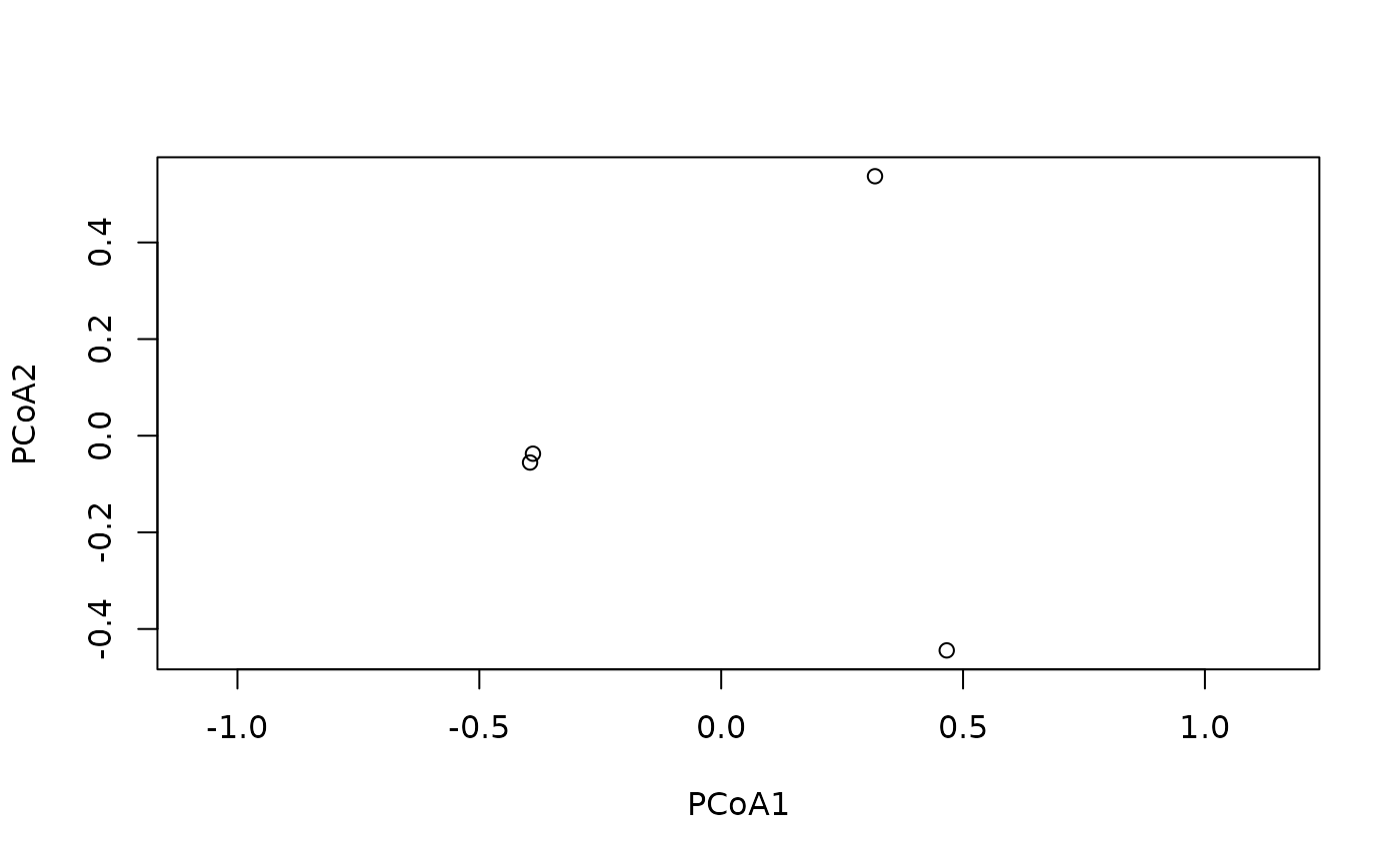
    ord <- pcoa(bray(ex_counts))
    ord
#>             PCoA1       PCoA2        PCoA3
#> Saliva -0.3891250 -0.03721713  0.296748867
#> Gums   -0.3951099 -0.05550727 -0.293514268
#> Nose    0.3179676  0.53707433 -0.006811864
#> Stool   0.4662673 -0.44434993  0.003577264
#> attr(,"method")
#> [1] "pcoa"
#> attr(,"eig")
#> [1] 0.6260388 0.4903619 0.1742697
#> attr(,"prop")
#> [1] 0.4850493 0.3799280 0.1350226
#> attr(,"trace")
#> [1] 1.29067

    # Percent of variance explained by each axis.
    round(100 * attr(ord, 'prop'), 1)
#> [1] 48.5 38.0 13.5

    # Same coordinates as cmdscale(), up to the sign of each axis.
    cmdscale(bray(ex_counts), k = 3)
#>              [,1]        [,2]         [,3]
#> Saliva -0.3891250  0.03721713  0.296748867
#> Gums   -0.3951099  0.05550727 -0.293514268
#> Nose    0.3179676 -0.53707433 -0.006811864
#> Stool   0.4662673  0.44434993  0.003577264

    plot(ord[, 1:2], asp = 1)