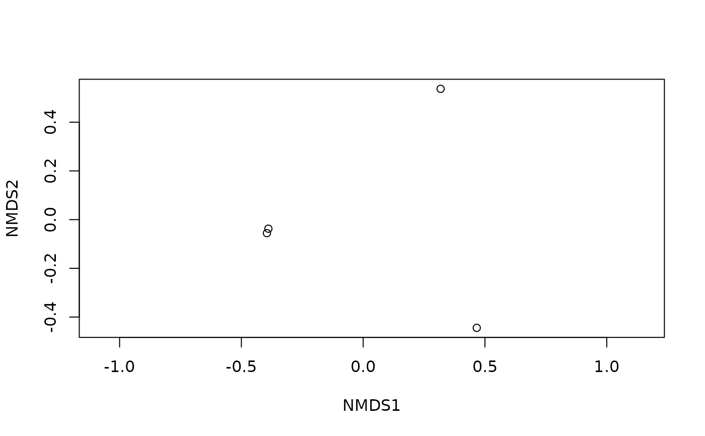
Ordinates samples from their distances, for plotting beta diversity, by
placing them so that their distances on the plot are in the same rank order
as the distances in dm, as nearly as possible. Follows the same procedure
as vegan::metaMDS() with its default monoMDS() engine, and gives the
same solutions from the same starting configurations, but runs the random
starts in parallel C with far less memory.
Usage
nmds(
  dm,
  k = 2L,
  try = 20L,
  trymax = 20L,
  maxit = 200L,
  weakties = TRUE,
  stress = 1L,
  smin = 1e-04,
  sfgrmin = 1e-07,
  sratmax = 0.999999,
  seed = 0L,
  cpus = n_cpus()
)
Arguments
- dm
A
distobject, such as frombeta_div()orbray(), or a symmetric numeric matrix of distances. Must not containNAs.- k
The number of dimensions. Default:
2- try, trymax
The minimum and maximum number of random starts. Random starts continue past
tryuntil the best solution is found again, ortrymaxis reached. Default:20and20- maxit
The maximum number of iterations for each start. Default:
200- weakties
How to treat tied distances in
dm.TRUE, the default, lets them have different distances on the plot (Kruskal's primary approach);FALSErequires their plot distances to be equal too (secondary approach).- stress
Kruskal's stress formula to minimize:
1(the default) or2.- smin, sfgrmin, sratmax
Each start stops when its stress falls below
smin, when the gradient's scale factor falls belowsfgrmin, or when the stress ratio between iterations rises abovesratmax(i.e., stress stops improving). Defaults:1e-4,1e-7and0.999999, as invegan::monoMDS().- seed
An integer seed for the random starting configurations. The same seed gives the same result. Default:
0- cpus
How many parallel processing threads should be used. The default,
n_cpus(), will use all logical CPU cores.
Value
A numeric matrix with one row per sample and one column per
dimension, named "NMDS1", "NMDS2", etc., as described in "Ordination
result" below. method is "nmds"; eig and prop are NA, as NMDS
has no eigenvalues. Then come:
stress: The stress of the solution (formulastress), from 0 (perfect) to 1.converged:TRUEif a random start found the best solution again.tries: The number of random starts run.best_try: Which start gave the solution:0for the PCoA start, else the random start's number.
Details
Method
NMDS minimizes Kruskal's stress: how far the distances between points
\(d_{ij}\) are from the closest sequence \(\hat{d}_{ij}\) that has the
same rank order as the distances in dm (found by monotone regression).
Formula 1 is
\(\sqrt{\sum(d_{ij} - \hat{d}_{ij})^2 / \sum d_{ij}^2}\); formula 2
divides by \(\sum(d_{ij} - \bar{d})^2\) instead.
Each start minimizes stress by steepest descent, with Kruskal's step-size
rules, as in Peter Minchin's monoMDS (the default engine of
vegan::metaMDS()). This is a line-by-line port of it, so from the same
starting configuration, a start gives exactly the same stress and
coordinates as vegan::monoMDS().
Steepest descent only finds a local minimum, so, as in metaMDS():
The first start is the PCoA solution, from
pcoa().Then come random starts, with coordinates uniform on [0, 1). A start whose stress is within 0.0005 of the best so far is compared with it by a Procrustes rotation; the best is "found again" when the root mean squared difference is below 0.005 and no point differs by more than 0.01. At least
tryrandom starts are run, and more, up totrymax, until the best is found again.The best solution is centered, rotated to its principal components, and scaled so that its largest distance equals the largest distance in
dm. Whendmhas amaxdistattribute (as fromvegan::vegdist()), it is instead scaled to half-change units, as invegan::postMDS().
Speed and memory
metaMDS() and monoMDS() copy dm into an \(n \times n\) matrix, and
keep several arrays with an element for every pair of samples, for every
start. nmds() sorts the pairs once, into one shared array of 4 bytes per
pair, and each start that runs at the same time needs about 16 more bytes
per pair. cpus starts run at once, each on its own thread.
Differences from metaMDS()
The random starting configurations come from
seed, not from R's random number generator, soset.seed()has no effect, and R's random number stream is left untouched. They differ from the onesmetaMDS()draws, so when there are several local minima of similar stress, the two can settle on different ones.The first start comes from
pcoa()rather thancmdscale(). The two differ only by rounding (about \(10^{-15}\)), butmonoMDS's stopping rule can react to that by stopping an iteration earlier or later, which changes the stress in about the 7th significant digit.Only
monoMDS's default "global" model is offered, not its "local", "linear", or "hybrid" ones.metaMDS()given a community matrix, asphyloseq::ordinate()does, first transforms the counts and computes the distances itself. Givenmds()those same distances to get the same solution.
Reproducibility
Results are identical from run to run and for any number of cpus.
Axes are flipped so that each one's coordinate with the largest absolute value is positive.
k larger than \(n - 1\) is reduced to \(n - 1\). A stress below
0.001 gives a warning, as in metaMDS(): there may be too few samples for
k dimensions.
Ordination result
Every ordination method (pcoa(), nmds(), and ordination()) returns
the same kind of object: a plain numeric matrix with one row per sample
(named after the samples) and one column per axis (named "PCoA1",
"NMDS1", etc.), so that it can go straight into plot() or a data
frame. Its attributes always begin with these three, in this order:
method: The method's ID, e.g."pcoa"or"nmds".eig: Each axis's eigenvalue, orNAfor methods without them.prop: The proportion of the total variance that each axis explains, orNAwhere that isn't defined.
Attributes particular to the method follow them.
References
Kruskal, J. B. (1964). Nonmetric multidimensional scaling: A numerical method. Psychometrika, 29(2), 115-129. doi:10.1007/BF02289694
Minchin, P. R. (1987). An evaluation of the relative robustness of techniques for ecological ordination. Vegetatio, 69, 89-107. doi:10.1007/BF00038690
Examples
    ord <- nmds(bray(ex_counts))
#> Warning: stress is (nearly) zero: there may be too few samples
    ord
#>             NMDS1       NMDS2
#> Saliva -0.3891463 -0.03721917
#> Gums   -0.3951316 -0.05551031
#> Nose    0.3179851  0.53710375
#> Stool   0.4662929 -0.44437427
#> attr(,"method")
#> [1] "nmds"
#> attr(,"eig")
#> [1] NA NA
#> attr(,"prop")
#> [1] NA NA
#> attr(,"stress")
#> [1] 0
#> attr(,"converged")
#> [1] FALSE
#> attr(,"tries")
#> [1] 20
#> attr(,"best_try")
#> [1] 0

    attr(ord, 'stress')
#> [1] 0

    plot(ord, asp = 1)