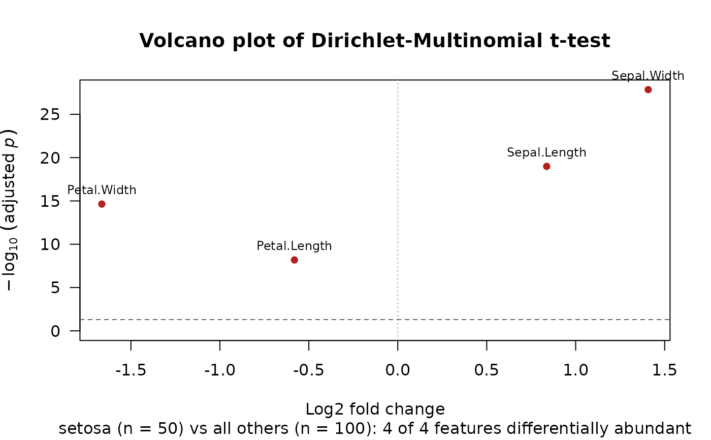
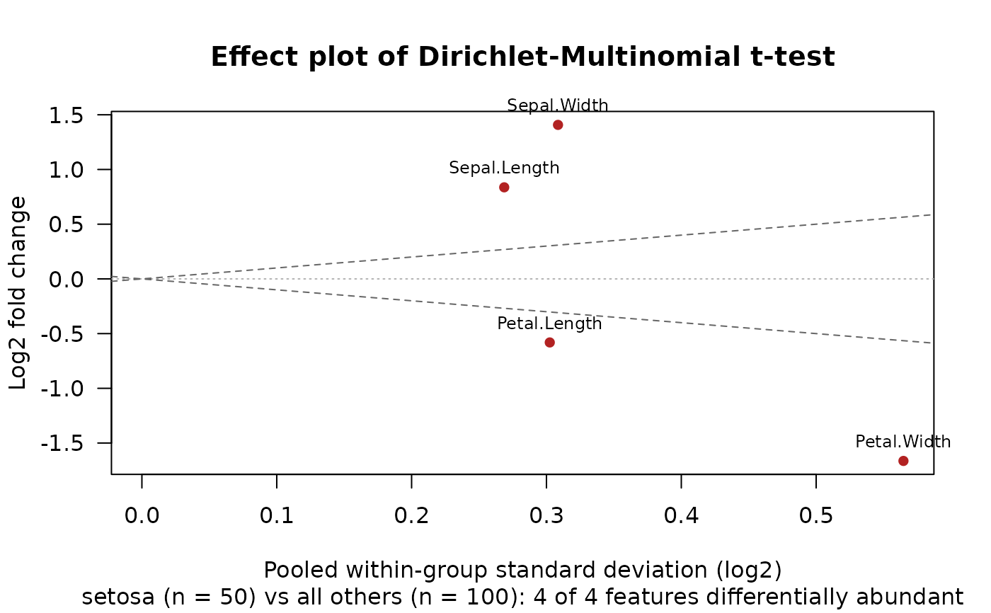
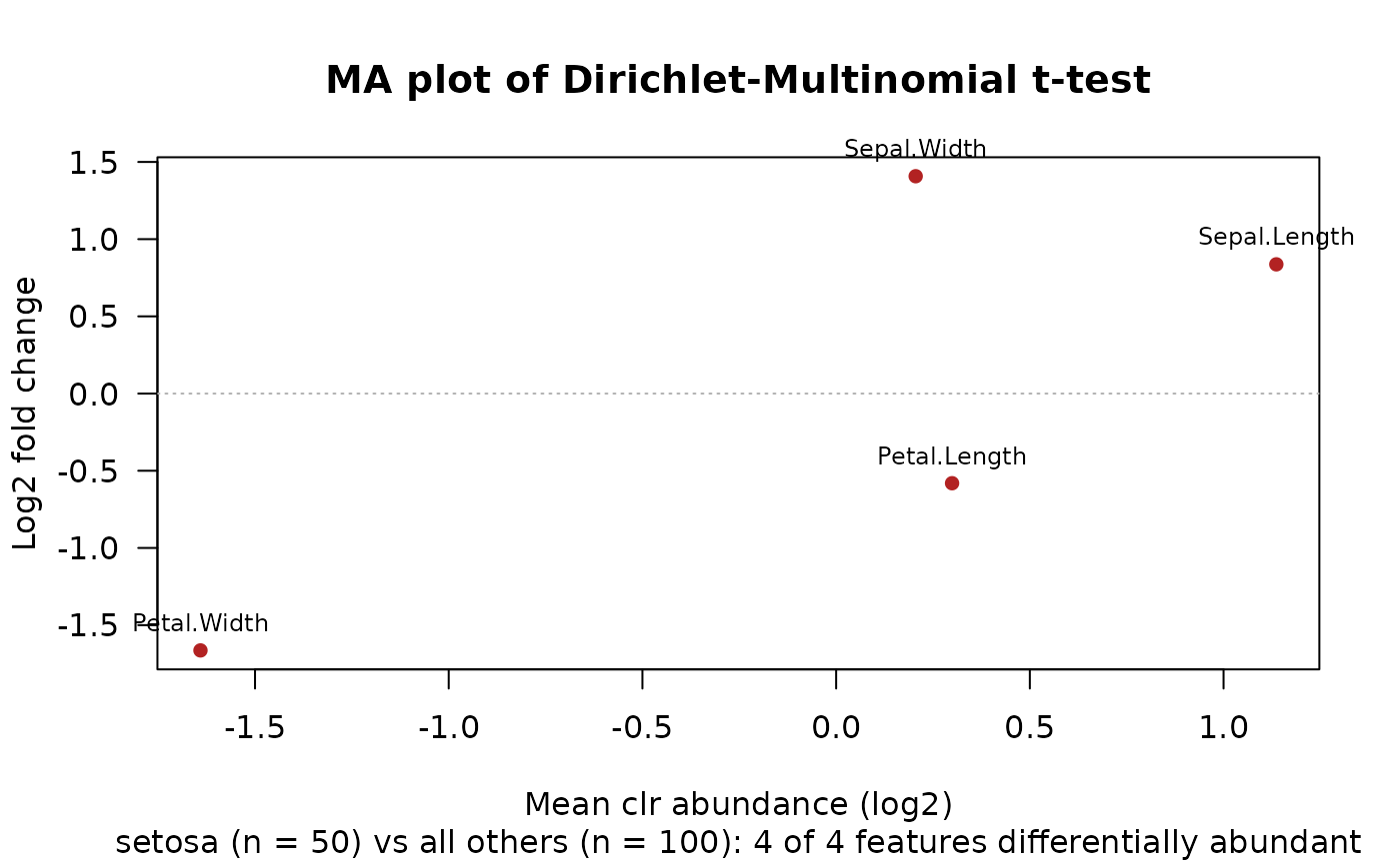
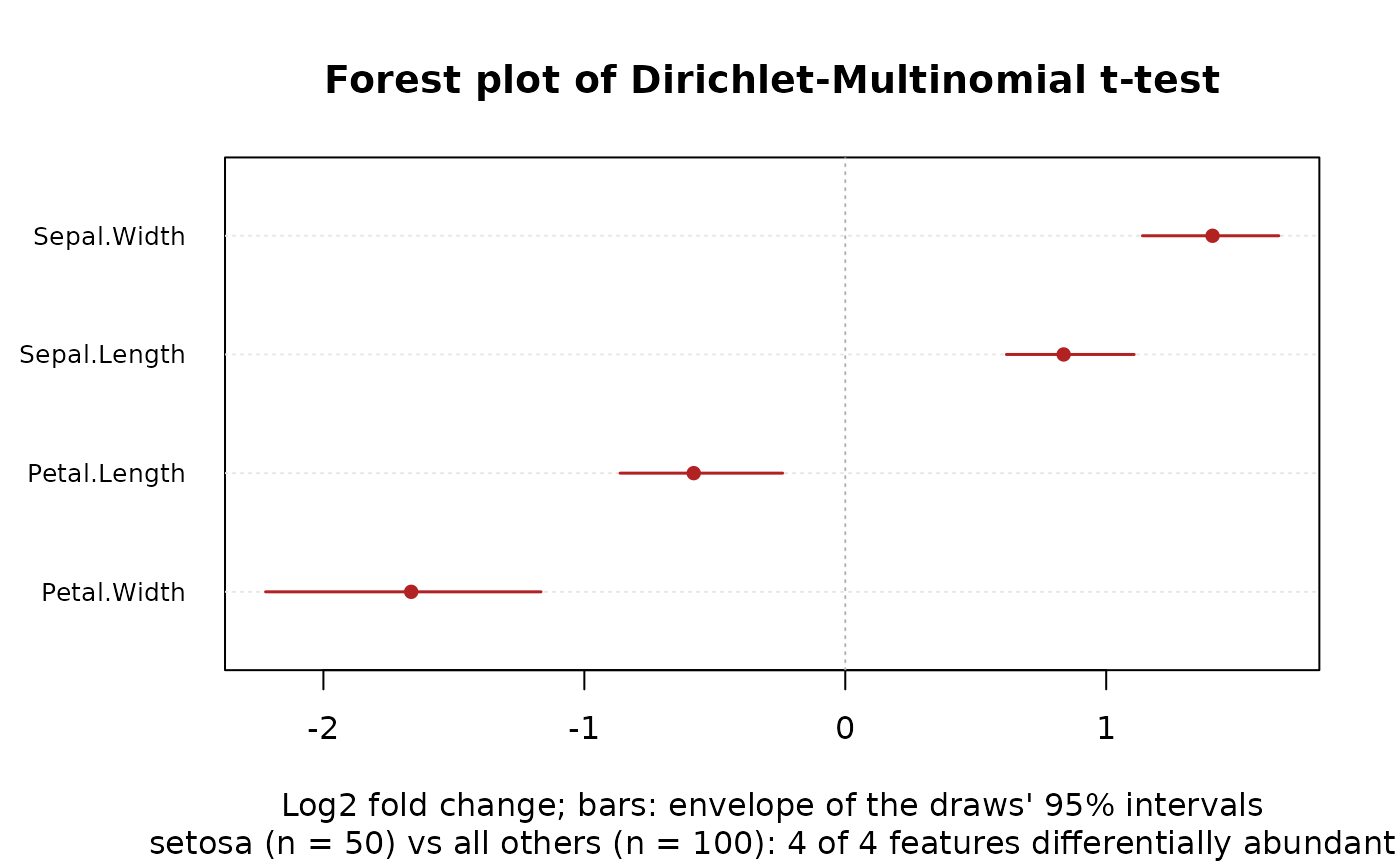
Four views of dirmult_ttest()'s results, each feature a point (or a
row), with the features that differ (reject = TRUE) highlighted and
the most significant of them named:
Arguments
- x
The result of
dirmult_ttest().- type
The plot:
"volcano"(the default),"effect","ma", or"forest".- labels
How many of the differentially abundant features to name (in the volcano, effect and MA plots), those with the smallest adjusted p-values. Default
10;0for none.- n_features
For
"forest": how many features to show, those with the smallest adjusted p-values (ties in the table's order). Default30;Inffor all.- ...
Passed on to
graphics::plot.default(), such asmain,sub,xlab,xlimorcex.
Details
"volcano"(the default): the log2 fold change against the adjusted p-value."effect": the log2 fold change against the pooled within-group standard deviation (Gloor et al. 2016; ALDEx2's"MW"plot)."ma": the log2 fold change against the mean clr abundance (ALDEx2's"MA"plot)."forest": the log2 fold changes and their intervals of then_featuresmost significant features, largest at the top.
Volcano plot. The y axis is \(-\log_{10}\) of p_adjusted (an
adjusted p-value of 0 is drawn at the smallest positive double). The
dashed line marks alpha; a feature also needs its interval for the
log2 fold change to exclude 0 to count as differentially abundant, so
some features above the line may not be highlighted. Gloor et al.
(2016) argue that volcano plots mislead: with many samples, tiny
differences reach small p-values, so read them with the effect plot.
Effect plot. Each feature's difference between the groups (y,
log2_fc) against its dispersion within them (x, pooled_sd), both in
log2 units. The dashed lines are \(y = \pm x\): features beyond them
differ between the groups by more than they vary within them (an
average effect of about 1 or more). Features near the y axis vary
little, so a small difference can be significant; features far to the
right need a large difference. This is ALDEx2's aldex.plot(type = "MW"), with ALDEx3's pooled standard deviation in place of ALDEx2's
diff.win (see dirmult_ttest()'s Effect sizes).
MA plot. The log2 fold change against the feature's mean clr value
(mean): how the differences depend on abundance. Rare features (on
the left) vary most, from sampling alone.
Forest plot. A point at each feature's log2_fc and a bar from
ci_lower to ci_upper, which are the envelope of the draws'
intervals (the lowest lower and highest upper bound), not an interval
of one draw: wider than a single confidence interval.
Features whose value is NaN are left out of each plot. The subtitle
names the contrast and counts the features rejected.
References
Gloor, G. B., Macklaim, J. M., & Fernandes, A. D. (2016). Displaying variation in large datasets: plotting a visual summary of effect sizes. Journal of Computational and Graphical Statistics, 25, 971-979. doi:10.1080/10618600.2015.1131161