
Runs any of ecodive's distance-based ordination methods by name, as
beta_div() does for beta diversity metrics and dist_test() does for
statistical tests. Compute the distances once with beta_div() (or a
metric's own function, such as bray()), then pass them to dist_ord()
and dist_test().
Arguments
- dm
The distances to ordinate: a
distobject such as frombeta_div(), or a symmetric matrix of distances. Every method listed bylist_dist_ords()takes distances.- method
The name of an ordination method:
"capda","capscale","dbrda","isomap","mds","nmds","pcoa","tsne", or"umap". Flexible matching is supported (see below). Programmatic access vialist_dist_ords().- ...
Further arguments for the method's function, such as
n_axes,seed,cpus, orpcoa'scorrection. Each method keeps its own defaults; seecapscale()anddbrda()(which also needgroups, ordataandformula, as indist_ord(dm, 'dbrda', 'treatment', meta)),capda()(which needsgroups, anddataifgroupsnames a column of it),isomap(),mds(),nmds(),pcoa(),tsne(), andumap().seedis ignored by the methods that have no random parts (capscale,dbrda,isomapandpcoa), so the same arguments can be given to every method.
Value
The method's result, as described in "Ordination result" below.
dist_ord(dm, 'pcoa', ...) is the same as pcoa(dm, ...).
Details
List of Ordination Methods
| Option / Function Name | Method Name |
capda | Discriminant Canonical Analysis of Principal Coordinates (CAP), supervised |
capscale | Constrained Analysis of Principal Coordinates |
dbrda | Distance-based Redundancy Analysis (db-RDA) |
isomap | Isometric Feature Mapping (Isomap) |
mds | Metric Multidimensional Scaling (MDS) |
nmds | Non-metric Multidimensional Scaling (NMDS) |
pcoa | Principal Coordinates Analysis (PCoA) |
tsne | t-distributed Stochastic Neighbor Embedding (t-SNE) |
umap | Uniform Manifold Approximation and Projection (UMAP) |
pca(), rda(), cca(), ca() and rpca() ordinate a count table rather than
distances, so they are run by count_ord(), or called directly. PCA is PCoA of Euclidean
distances: dist_ord(euclidean(counts), 'pcoa') gives the same scores as
pca(counts), up to each axis's sign, but pca() also returns the
features' loadings and never forms the distance matrix. permanova() and
ecodive's other tests are run by dist_test().
Default numbers of axes differ: n_axes = 3 for the methods whose axes
have eigenvalues (capscale, dbrda, isomap, pcoa, and pca() and
rpca(); capda returns up to 3, and at most one fewer than the number
of groups), and n_axes = 2 for those that fit a layout in a fixed number
of dimensions (mds, nmds, tsne, and umap).
Flexible name matching
Case insensitive and partial matching, ignoring anything but letters. E.g.
method = 'PCoA' or 'principal coord' selects pcoa. Common other names
also work: 'PCO', 'cmdscale', or 'classical MDS' for pcoa;
'MDS' or 'metric MDS' for mds; 'non-metric MDS', 'metaMDS',
'monoMDS', or 'isoMDS' for nmds; 'isometric mapping' for isomap;
'Rtsne', 'bhtsne', or 'Barnes-Hut t-SNE' for tsne; and 'uwot'
for umap. 'dbRDA' or 'distance-based RDA' select dbrda, and 'CAP'
selects capscale (but 'CA' names ca(), which takes a count table).
'CAPdiscrim' (BiodiversityR's name) or 'discriminant CAP' select
capda, Anderson & Willis's discriminant CAP.
Finished code should always use the full primary option name to avoid ambiguity with future additions to the list of methods.
Same names in other packages
ape::pcoa(), vegan::pca(), vegan::dbrda(), vegan::capscale(),
vegan::isomap() (whose k is the number of neighbours, not axes), and
uwot::umap() share names with ecodive's functions, and whichever package was attached last
masks the other's. Write ecodive::pcoa() and so on, or use
dist_ord(), which always runs ecodive's, to be sure.
Ordination result
Every ordination function (pcoa(), pca(), rpca(), dbrda(), capda(),
capscale(), mds(), nmds(), isomap(), tsne(), umap(), and so
dist_ord()) returns the same kind of
object: a numeric matrix with one row per sample and one column per
axis, so that it can go straight into a data frame. Rows are
named after the samples, when the input has names. Columns are named
after the method: "PCoA1", "PC1", "RPCA1", "dbRDA1" or "CAP1"
(then "MDS1" for unconstrained axes), "MDS1", "NMDS1",
"Isomap1", "TSNE1", "UMAP1", and so on.
Its attributes always begin with these three, in this order, each with one value per column:
method: The method's ID, e.g."pcoa"or"nmds".eig: Each axis's eigenvalue, on the method's own scale:pcoa()andisomap()give the eigenvalues of Gower's centered matrix (sums of squares);pca()andrpca()give variances, which arepcoa()'s divided by \(n - 1\) for \(n\) samples; anddbrda()andcapscale()followvegan, which also divides by \(n - 1\) when any distance is 4 or more.NAformds(),nmds(),tsne(), andumap(), which have no eigenvalues.prop: The proportion of the total variance (or inertia) that each axis explains. Unlikeeig, it is comparable between methods, so use it to label axes.NAwhere it isn't defined.
Attributes particular to the method follow them, and last display,
with the ordination's title for plot() and print(): the method's
name, and for the methods that take distances, the distance matrix's
title, such as "Principal Coordinates Analysis of Bray-Curtis
Dissimilarity" (see ecodive_display). The matrix has class
"ecodive_ord" (as well as "matrix"), so that print() lists the
other attributes by name rather than in full, and plot() draws the
samples on the first two axes, labelled from the attributes, with any
loadings, constraints and centroids on top (see plot.ecodive_ord()).
plot(ord, "Species", iris) colours the samples by a column of
metadata. Subsetting with [, or as.data.frame(), gives a plain
matrix or data frame without the attributes.
See also
capda(), capscale(), dbrda(), isomap(), mds(), nmds(), pcoa(),
tsne(), umap(), list_dist_ords(); count_ord() for pca(),
rda(), cca(), ca() and rpca(), which take a count table; dist_test() for
ecodive's tests.
Examples
dm <- bray(iris[, 1:4])
ord <- dist_ord(dm, 'pcoa')
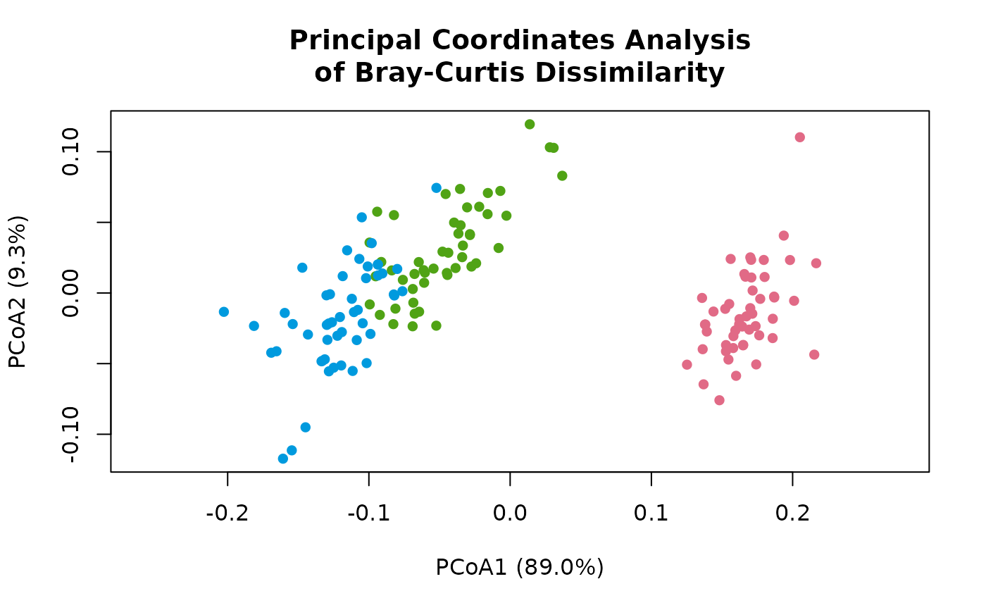
plot(ord, 'Species', iris)
 ord
#> # A matrix: 150 samples × 3 axes
#> # Principal Coordinates Analysis of Bray-Curtis Dissimilarity
#> # % of variance: 89.0, 9.3, 2.9
#> PCoA1 PCoA2 PCoA3
#> 1 0.169 -0.0259 -0.00505
#> 2 0.171 0.0235 0.0308
#> 3 0.187 -0.0032 0.0322
#> 4 0.18 0.0113 0.0372
#> 5 0.176 -0.03 -0.00613
#> 6 0.136 -0.0398 -0.0431
#> 7 0.186 -0.0182 0.0156
#> 8 0.167 -0.0165 0.00287
#> 9 0.194 0.0406 0.0413
#> 10 0.171 0.011 0.0286
#> # … 140 more samples
#> # Use print(x, n = ...) to see more samples
#> # Attributes: method, eig, prop, trace, correction, constant
str(ord)
#> 'ecodive_ord' num [1:150, 1:3] 0.169 0.171 0.187 0.18 0.176 ...
#> - attr(*, "dimnames")=List of 2
#> ..$ : NULL
#> ..$ : chr [1:3] "PCoA1" "PCoA2" "PCoA3"
#> - attr(*, "method")= chr "pcoa"
#> - attr(*, "eig")= num [1:3] 2.3473 0.2459 0.0766
#> - attr(*, "prop")= num [1:3] 0.8901 0.0932 0.0291
#> - attr(*, "trace")= num 2.64
#> - attr(*, "correction")= chr "none"
#> - attr(*, "constant")= num 0
#> - attr(*, "display")=List of 1
#> ..$ title: chr "Principal Coordinates Analysis of Bray-Curtis Dissimilarity"