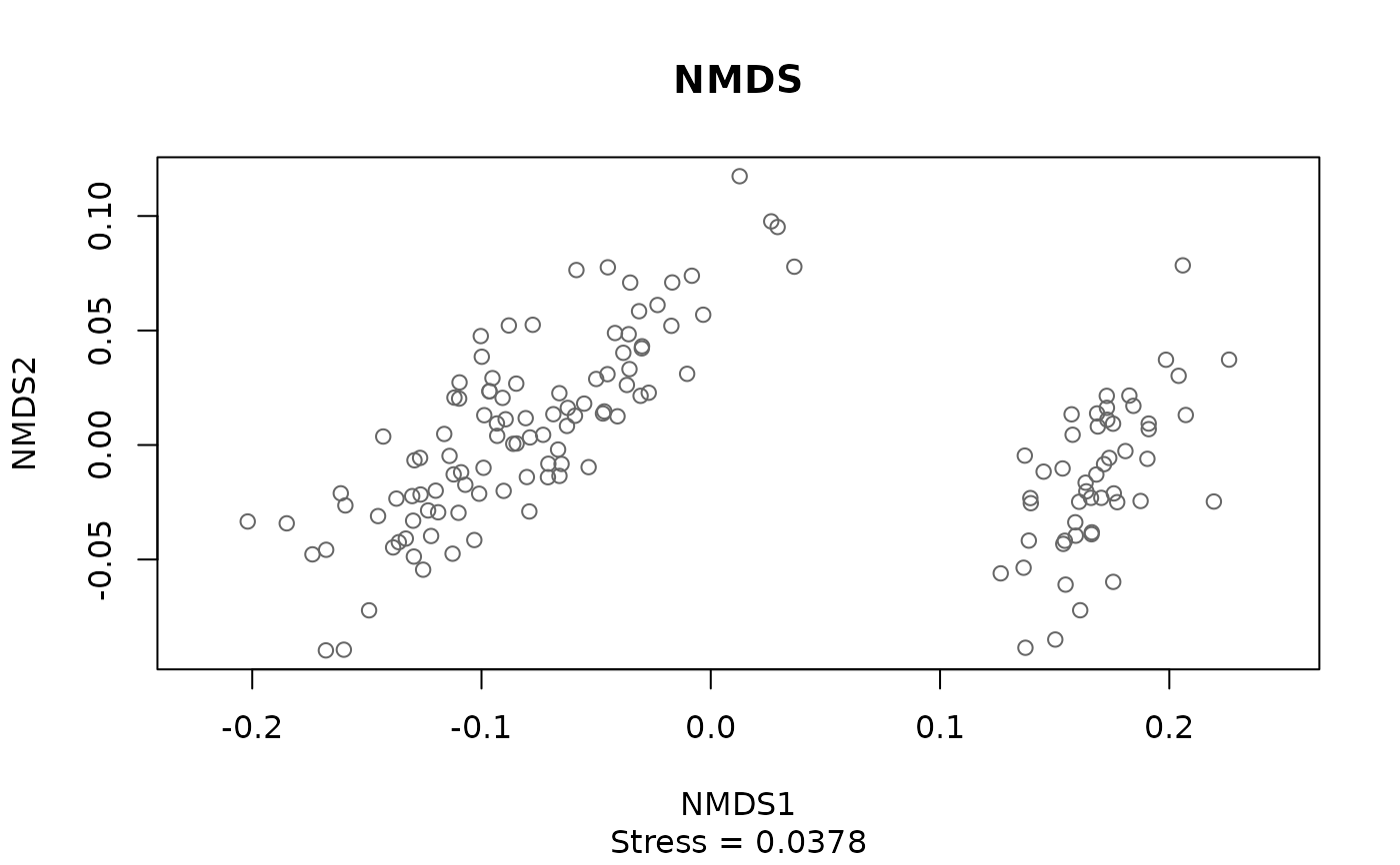
Draws the samples on two axes of an ordination from pcoa(), pca(),
dbrda(), procrustes() or any other of ecodive's ordination methods,
with the title, axis labels and subtitle taken from the result's
attributes. The overlays the result holds are drawn on top of the samples:
feature loadings, the arrows of numeric constraints, factor or group
centroids, and the target of a Procrustes rotation. Nothing is recomputed:
this is a quick look at results already in hand.
Arguments
- x
An ordination result: a matrix of class
ecodive_ord, fromdist_ord(),count_ord(),pcoa(),mds(),nmds(),isomap(),tsne(),umap(),dbrda(),capscale(),rda(),cca(),ca(),pca(),rpca(),rpca_phylo(),lda(),plsda(),oplsda(), orprocrustes().- groups
Colours the samples by group, with a legend: the name of a column of
data, or a vector with one value per sample (matched to the samples by name when both are named, as forpermanova()). A factor, character or logical vector gives each value its own colour, in the order of a factor's levels; a numeric vector gives a colour gradient (convert it withfactor()for one colour per value). A factor's unused levels keep their colours, so that plots of subsets match, but are left out of the legend. By default, the groups thatlda(),plsda()andoplsda()store in theirgroupsattribute, if any.- data
A data frame of sample metadata, with one row per sample (matched by row name, else in order), when
groupsnames one of its columns.- axes
Which two axes to plot, by number, as in
envfit(). Defaultc(1, 2). A result with only one axis (such aslda()of two groups) is drawn as a strip chart, with one strip per group (in which caseaxesis not used).- loadings
How many of the features in the
loadingsattribute to draw, those furthest from the origin on the plotted axes first: a number,Inf(orTRUE) for all, or0(orFALSE) for none. Default10. Drawn as arrows forpca(),rpca(),rpca_phylo(),rda(),plsda()andoplsda(), and as labelled points for the species scores ofca()andcca().- biplot
Whether to draw the arrows of the constraints in the
biplotattribute ofdbrda(),capscale(),rda()andcca(). Those of factor levels are left out whencentroidsare drawn. DefaultTRUE.- centroids
Whether to label the points in the
centroidsattribute: the centroid of each factor level of a constrained ordination, or of each group ofplsda()andoplsda(). DefaultTRUE. Those of the plottedgroupsare labelled with the group and drawn in its colour.- target
For
procrustes(), whether to draw an arrow from each sample to its place in thetargetattribute, the ordination it was fitted to. DefaultTRUE.- legend
Where to put the legend of
groups: a keyword forgraphics::legend(), such as"topright"(the default) or"bottomleft", orNULLfor none.- col
The points' colours. Without
groups, passed toplot()as given, so thatcol = iris$Speciesworks as for any matrix. Withgroups, one colour per group (in order, or named by group); for numericgroups, the colours of the gradient, from low to high. Defaults togrDevices::hcl.colors()'s"Dark 3"palette for groups and its"Viridis"palette for a gradient.- pch
The points' symbols, as for
plot(). Default1(open circles), or16(filled circles) withgroups.- ...
Passed on to
graphics::plot.default(), such asmain,sub,xlab,xlim,asporcex. They replace the defaults made fromx. To leave out the axes, usexaxt = "n"andyaxt = "n", sinceaxeschooses which axes to plot.
Details
The plot is made of what x holds:
Title: the ordination's title (see ecodive_display): the method's name, as
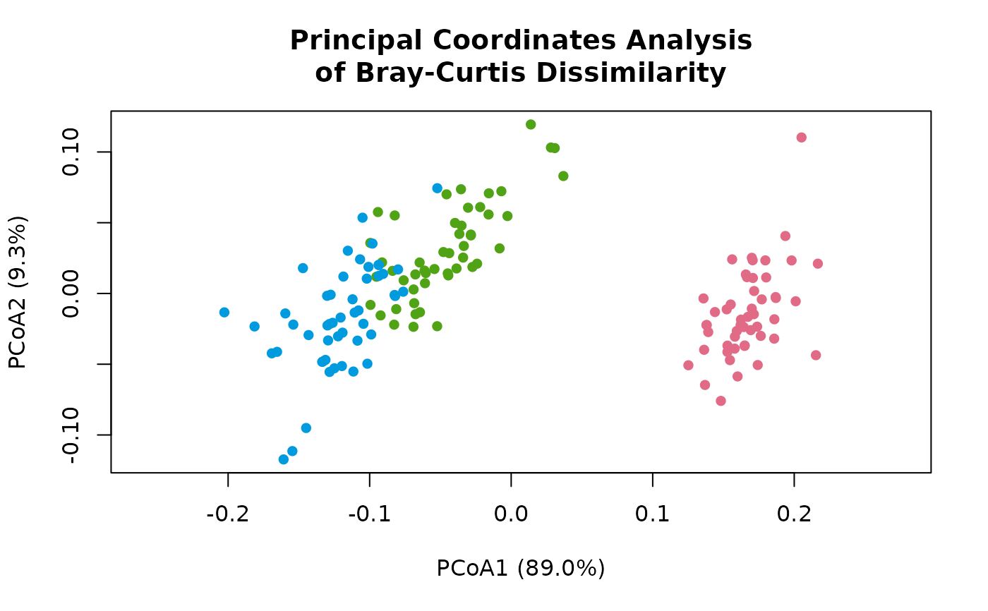
list_dist_ords()andlist_count_ords()give it, and for an ordination of distances, the distances' metric, such as "Principal Coordinates Analysis of Bray-Curtis Dissimilarity".Axis labels: the axes' names, with the percentage of the variance each explains (the
propattribute), for methods that have one.Subtitle: how well the method fit, for methods that measure it: the
stressofmds()andnmds(), thekl_divergenceoftsne(), the \(R^2\) (r_squaredandadj_r_squared) of a constrained ordination,r2xandr2yofoplsda(), and thessofprocrustes(); and forpcoa(),isomap()andumap(), their settings.
The axes have the same scale (asp = 1), so that distances on the plot
are true to the ordination; give asp = NA to let each axis fill the
plot.
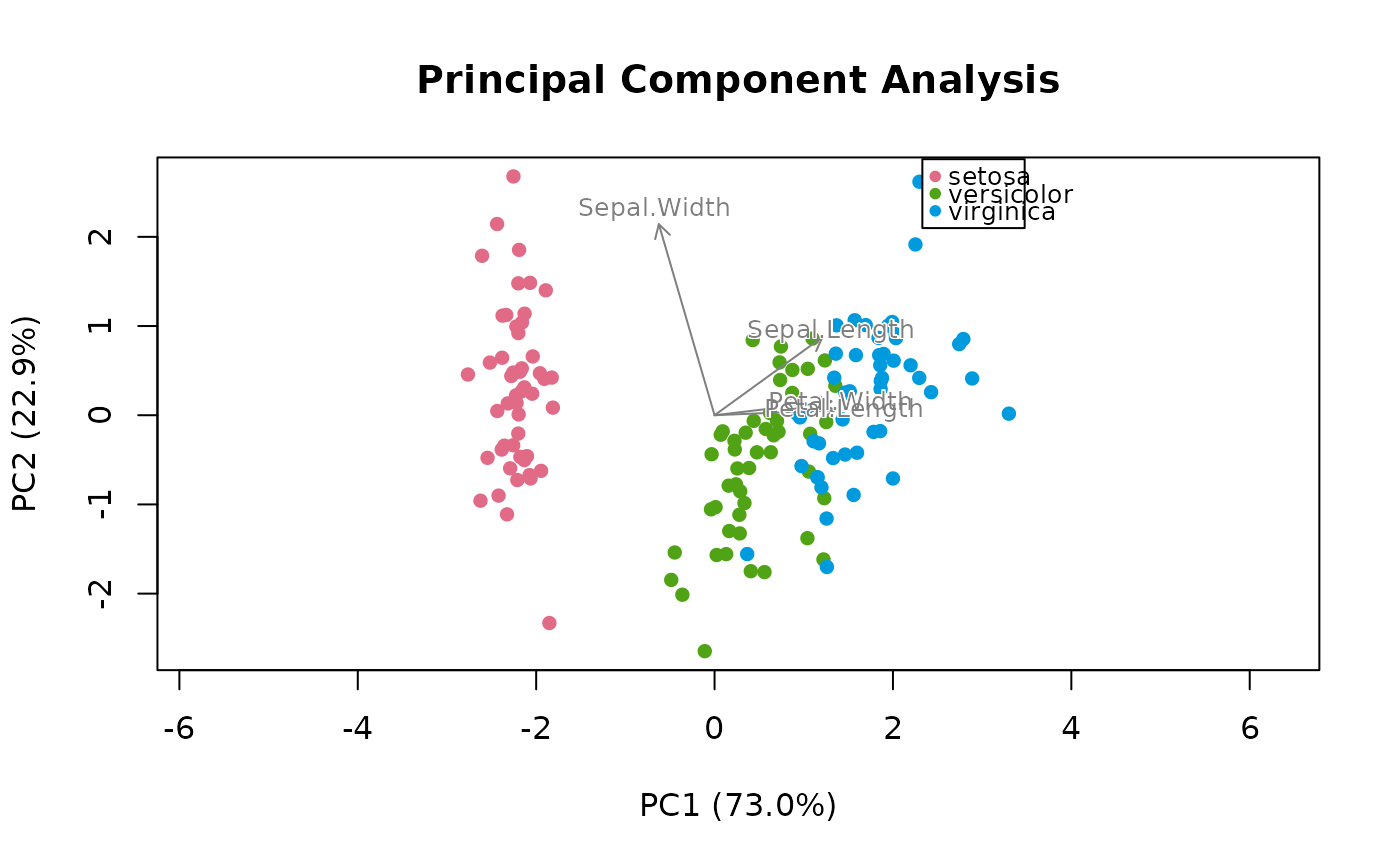
Arrows (loadings and constraints) are scaled to fit among the samples, as
in any biplot: only their directions and relative lengths have meaning.
Loadings and constraints are scaled separately. Centroids, and the
species scores of ca() and cca() (vegan's scaling 2), are drawn
where they are.
Base graphics draw on the current device, so further points, text or
arrows can be added on top. Use envfit()'s plot method, plot(fit, add = TRUE), to add fitted variables.
See also
envfit() and its plot method, plot(fit, add = TRUE), to add
fitted variables to an ordination plot.
Examples
# Colour by a column of metadata, with a legend.
ord <- pcoa(bray(iris[, 1:4]))
plot(ord, 'Species', iris)
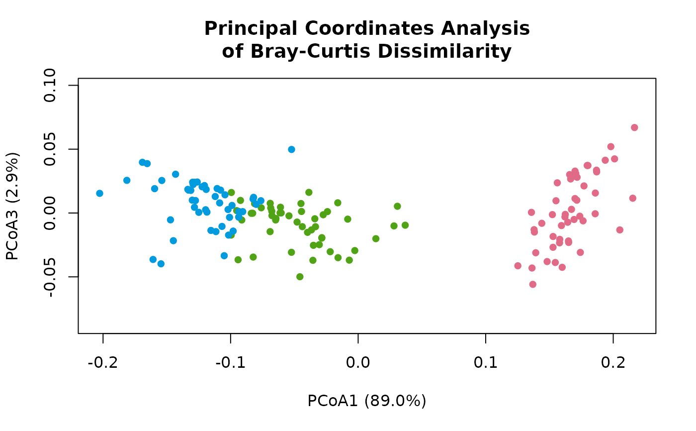
 # The third axis instead of the second.
plot(ord, 'Species', iris, axes = c(1, 3))
 # A PCA biplot: the loadings as arrows.
plot(pca(iris[, 1:4], scale = TRUE), iris$Species)
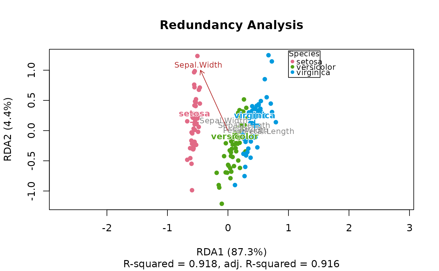
 # A constrained ordination: centroids of each species, and an arrow
# for the numeric constraint.
ord <- rda(iris[, 1:4], data = iris, formula = ~ Species + Sepal.Width)
plot(ord, 'Species', iris)
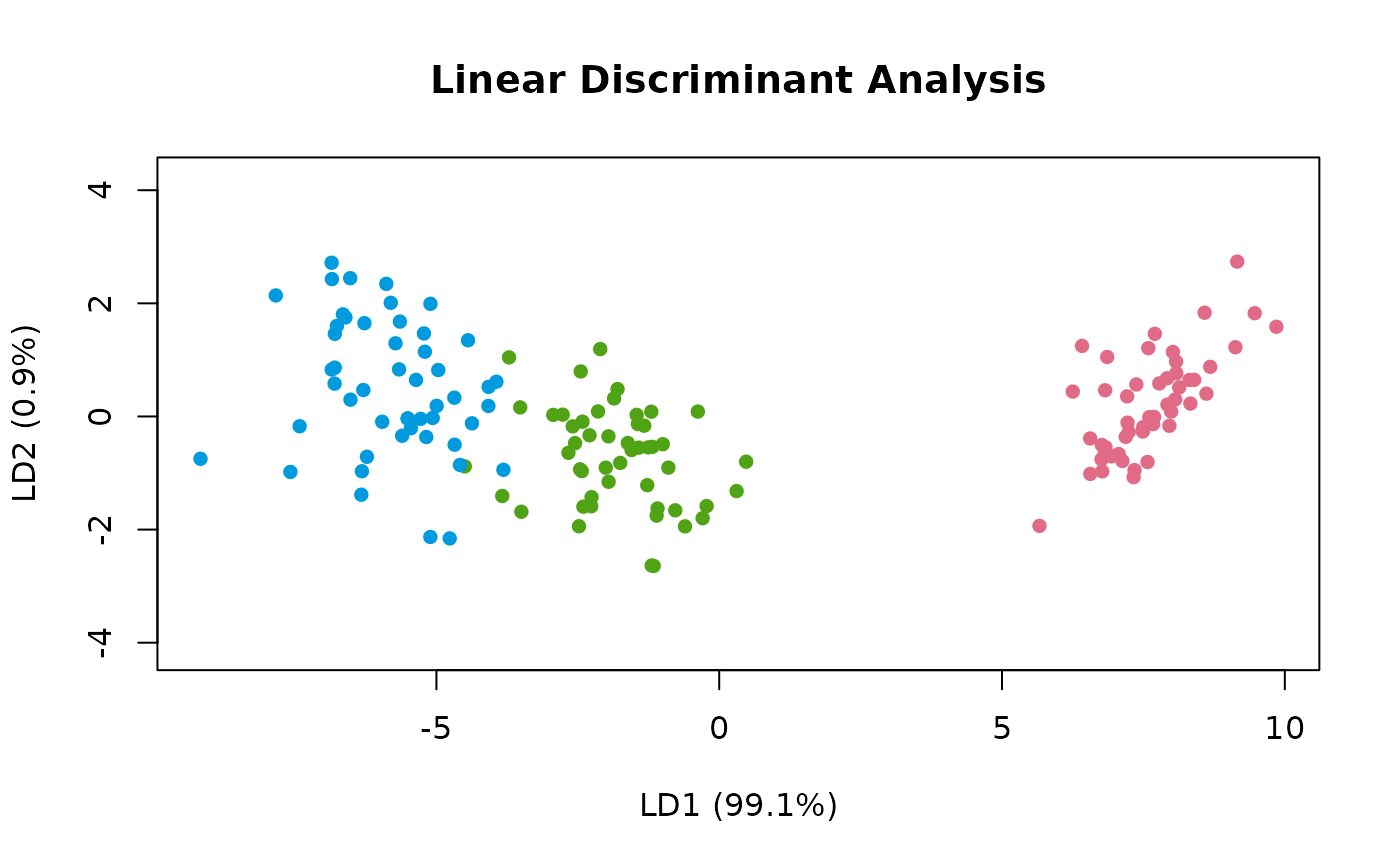
 # Supervised methods colour by their own groups.
plot(lda(iris[, 1:4], 'Species', iris))
 # Any argument of plot() still works.
plot(nmds(bray(iris[, 1:4]), seed = 1), col = 'grey40', main = 'NMDS')