
Supervised ordination of samples from their feature abundances: the
components of a (normalized) count table that best separate known groups.
PLS-DA is partial least squares (PLS) regression of a dummy matrix of the
groups on the table. Gives the same results as scikit-learn's
PLSRegression and mixOmics::plsda(), computed straight from sparse
input without forming any dense table or \(n \times n\) matrix.
Usage
plsda(
  counts,
  groups,
  data = NULL,
  margin = 1L,
  norm = "none",
  pseudocount = NULL,
  scale = TRUE,
  n_axes = 2L,
  cpus = n_cpus()
)
Arguments
- counts
A numeric matrix of feature abundances (samples \(\times\) features), or any of the table types listed under "Input Types".
- groups
The known group of each sample: a vector or factor with one value per sample, matched to the samples in
countsby name when both are named, else in the same order. Or, whendatais given, the name of one of its columns (or a vector with one value per row ofdata). Every distinct value is a group, numbers included; there must be at least two. A factor's unused levels are dropped.- data
Sample metadata: a data frame with one row per sample, holding the column named in
groups. Rows are matched to the samples incountsby row name, and rows for other samples are ignored; without row names, they must be in the same order as the samples. Default:NULL.- margin
The margin containing samples.
1if samples are rows,2if samples are columns. Ignored whencountsis a special object class (e.g.phyloseq). Default:1- norm
Normalize the incoming counts. Options are:
'none': No transformation.'percent': Relative abundance (sample abundances sum to 1).'hellinger': Square root of relative abundance (the Hellinger transformation).'binary': Unweighted presence/absence (each count is either 0 or 1).'clr': Centered log ratio.'rclr': Robust centered log ratio.'log': Log relative abundance (log-TSS), withpseudocountadded to every value first.
Default:
'none'.- pseudocount
Value added to counts to handle zeros when
norm = 'clr'or'log'. Ignored for other normalization methods. See Pseudocount section.- scale
Scale each feature to unit variance (after
norm, before the analysis), and each column of the dummy matrix too, as scikit-learn'sPLSRegression(scale = True)andmixOmics::plsda(scale = TRUE)do, so that every feature has equal weight. Features with constant values are left out: their weights, loadings and VIP are 0. Default:TRUE- n_axes
The number of components to return. Default:
2. Reduced to \(n - 1\) for \(n\) samples, or to the number of features, if fewer; and, with a warning, to the number of components that the table can fit (see "Method").- cpus
How many parallel processing threads should be used. The default,
n_cpus(), is the CPU cores this R process may use, within any limits set on it. Results are the same for anycpus.
Value
A numeric matrix with one row per sample and one column per
component, named "PLSDA1", "PLSDA2", etc., as described in
"Ordination result" below. The values are the X scores \(t\)
(scikit-learn's x_scores_, mixOmics' variates$X). Attributes:
method:"plsda".eig: The variance of the table that each component explains, \(|t|^2 |p|^2 / (n - 1)\) for scores \(t\) and loadings \(p\). (PLS components are not eigenvectors; this is the analogue ofpca()'s eigenvalues, and it adds up over components.)prop: The proportion of the table's total variance that each component explains,eig / trace:mixOmics'prop_expl_var$X.trace: The total variance of the table: the sum of all features' variances (afternormandscale), aspca()'strace.loadings: The X loadings \(p\): one row per feature and one column per component (scikit-learn'sx_loadings_). Each column regresses the (deflated) table on the component's scores.weights: The X weights \(w\), unit-length columns (scikit-learn'sx_weights_; whatmixOmicscallsloadings$X).y_loadings: The Y loadings \(q\): one row per group and one column per component (scikit-learn'sy_loadings_), for the dummy matrix as centred (and scaled).vip: Variable importance in projection (VIP): one row per feature, and one column per number of components, the column for \(a\) components counting the first \(a\) (asmixOmics::vip()). See "Method".groups: Each sample's group, as a factor whose levels are the groups, in the order of the rows ofy_loadingsandcentroids.centroids: The mean score of each group: one row per group and one column per component.
Details
Method
Let \(X\) be the normalized table, its features centred (and, with
scale = TRUE, scaled to unit variance), and \(Y\) the dummy matrix of
the groups (one column per group, 1 for that group's samples and 0 for
the others), centred (and scaled) the same way. PLS regression (Wold et
al. 2001) finds one component at a time. With \(X_a\) and \(Y_a\)
what is left of \(X\) and \(Y\) before component \(a\):
the weights \(w\) are the top left singular vector of \(X_a^T Y_a\), the direction in which \(X_a\) covaries most with \(Y_a\);
the scores are \(t = X_a w\);
the loadings are \(p = X_a^T t / |t|^2\) and the Y loadings \(q = Y_a^T t / |t|^2\);
both tables are deflated by the scores: \(X_{a+1} = X_a - t p^T\) and \(Y_{a+1} = Y_a - t q^T\) (regression mode).
Barker & Rayens (2003) give the link to discriminant analysis. Fitting stops early, with a warning, when \(X_a^T Y_a\) falls to \(\sqrt{\epsilon} \approx 1.5 \times 10^{-8}\) times its value for the first component: then what is left of the table has no covariance with the groups, beyond rounding error (for instance, once the components span the whole table).
VIP (Wold et al. 2001; Mehmood et al. 2012) sums each feature's squared
weights over the first \(a\) components, each weighted by the
component's share of the explained sum of squares of \(Y\),
\(SSY_b = |t_b|^2 |q_b|^2\):
$$VIP_j = \sqrt{P \sum_{b \le a} SSY_b w_{jb}^2 / \sum_{b \le a} SSY_b}$$
for \(P\) features (constant ones included, when scale leaves them
out). The mean of the squared VIPs is 1, so features with a VIP above 1
are often called important.
The table is never centred in memory: products with \(X_a\) are
computed from the non-zero values alone, in parallel, as in pca(), so
a sparse table is never made dense.
Choosing norm
For microbiome counts, norm = 'clr' (with a pseudocount) is the usual
choice, as in mixOmics' logratio = 'CLR': PLS-DA then works on
log-ratios, which suit compositional data.
Validate the separation
PLS-DA is supervised: it looks for the directions that separate the
groups, so its plots separate them even when the groups don't differ
(with more features than samples, almost always). Don't read the plot as
evidence of a difference. Test it with a permutation test of the
distances, such as permanova(), or estimate the error rate of
classifying new samples by cross-validation.
Matching scikit-learn and mixOmics
plsda() gives the same scores, weights, loadings and Y loadings as
scikit-learn's PLSRegression(n_components, scale = True) fitted to the
normalized table and the dummy matrix, up to the signs of the
components, and the same scores, weights (loadings$X), explained
variance (prop_expl_var$X) and VIP (mixOmics::vip()) as
mixOmics::plsda(). (With scale = FALSE, mixOmics::vip() weights each
component by its squared correlations with the dummy columns rather than
by \(SSY\), which is the same only when they are scaled; plsda()
keeps the textbook formula.) Both fit each component by NIPALS, a power iteration that converges to
the weights above; plsda() computes them directly instead, as
scikit-learn's algorithm = "svd" does, so it matches them when they
are run with a small tolerance (tol). With their default tolerances,
their results with three groups or more can differ from the converged
ones by about 0.1%. With two groups, NIPALS converges at once.
Same names in other packages
mixOmics::plsda() and caret::plsda() share their names with
ecodive's plsda(), and whichever package was attached last masks the
other's. Write ecodive::plsda(), or use count_ord(), which always runs
ecodive's, to be sure.
Component signs and reproducibility
A component's sign is arbitrary, so different software can return mirror
images of the same component. plsda() flips each component so that its
largest score in absolute value is positive, and flips its weights,
loadings and Y loadings with it. Results are identical from run to run
and for any number of cpus.
Ordination result
Every ordination function (pcoa(), pca(), rpca(), dbrda(), capda(),
capscale(), mds(), nmds(), isomap(), tsne(), umap(), and so
dist_ord()) returns the same kind of
object: a numeric matrix with one row per sample and one column per
axis, so that it can go straight into a data frame. Rows are
named after the samples, when the input has names. Columns are named
after the method: "PCoA1", "PC1", "RPCA1", "dbRDA1" or "CAP1"
(then "MDS1" for unconstrained axes), "MDS1", "NMDS1",
"Isomap1", "TSNE1", "UMAP1", and so on.
Its attributes always begin with these three, in this order, each with one value per column:
method: The method's ID, e.g."pcoa"or"nmds".eig: Each axis's eigenvalue, on the method's own scale:pcoa()andisomap()give the eigenvalues of Gower's centered matrix (sums of squares);pca()andrpca()give variances, which arepcoa()'s divided by \(n - 1\) for \(n\) samples; anddbrda()andcapscale()followvegan, which also divides by \(n - 1\) when any distance is 4 or more.NAformds(),nmds(),tsne(), andumap(), which have no eigenvalues.prop: The proportion of the total variance (or inertia) that each axis explains. Unlikeeig, it is comparable between methods, so use it to label axes.NAwhere it isn't defined.
Attributes particular to the method follow them, and last display,
with the ordination's title for plot() and print(): the method's
name, and for the methods that take distances, the distance matrix's
title, such as "Principal Coordinates Analysis of Bray-Curtis
Dissimilarity" (see ecodive_display). The matrix has class
"ecodive_ord" (as well as "matrix"), so that print() lists the
other attributes by name rather than in full, and plot() draws the
samples on the first two axes, labelled from the attributes, with any
loadings, constraints and centroids on top (see plot.ecodive_ord()).
plot(ord, "Species", iris) colours the samples by a column of
metadata. Subsetting with [, or as.data.frame(), gives a plain
matrix or data frame without the attributes.
Input Types
The counts parameter is designed to accept a simple numeric matrix, but
seamlessly supports objects from the following biological data packages:
phyloseqrbiomSummarizedExperimentTreeSummarizedExperiment
For large datasets, standard matrix operations may be slow. See
vignette('performance') for details on using optimized formats
(e.g. sparse matrices) and parallel processing.
Pseudocount
The pseudocount parameter is only relevant when norm = 'clr'
or norm = 'log'.
Zeros are undefined in the centered log-ratio (CLR) transformation and
in the log of proportions. If norm is 'clr' or
'log', pseudocount is NULL (the default), and
zeros are detected, the function uses half the minimum non-zero value
(min(x[x>0]) / 2) and issues a warning.
To suppress the warning, provide an explicit value (e.g., 1), or
replace the zeros first with replace_zeros(), whose
result needs no pseudocount.
Why this matters: The choice of pseudocount is not neutral; it acts as a weighting factor that can significantly distort downstream results, especially for sparse datasets. See Gloor et al. (2017) and Kaul et al. (2017) for open-access discussions on the mathematical implications, or Costea et al. (2014) for the impact on community clustering.
See aitchison for references.
References
Wold, S., Sjöström, M., & Eriksson, L. (2001). PLS-regression: a basic tool of chemometrics. Chemometrics and Intelligent Laboratory Systems, 58(2), 109-130. doi:10.1016/S0169-7439(01)00155-1
Barker, M., & Rayens, W. (2003). Partial least squares for discrimination. Journal of Chemometrics, 17(3), 166-173. doi:10.1002/cem.785
Mehmood, T., Liland, K. H., Snipen, L., & Sæbø, S. (2012). A review of variable selection methods in partial least squares regression. Chemometrics and Intelligent Laboratory Systems, 118, 62-69. doi:10.1016/j.chemolab.2012.07.010
Pedregosa, F., et al. (2011). Scikit-learn: machine learning in Python. Journal of Machine Learning Research, 12, 2825-2830.
Examples
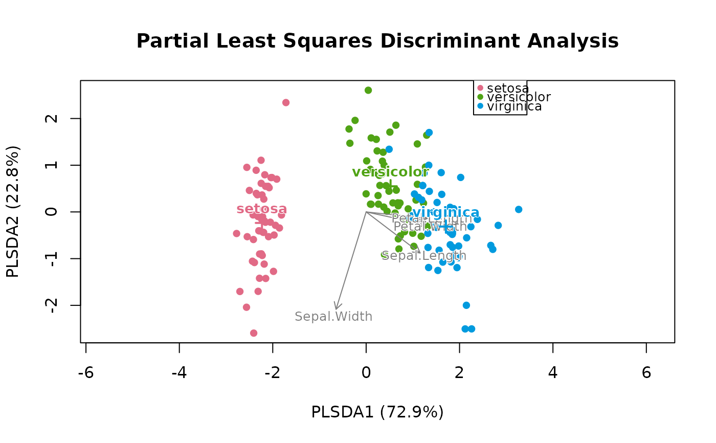
# PLS-DA of iris, as if its measurements were counts.
counts <- round(iris[, 1:4] * 10)
ord <- plsda(counts, 'Species', iris)
ord
#> # A matrix: 150 samples × 2 axes
#> # Partial Least Squares Discriminant Analysis
#> # % of variance: 72.9, 22.8
#> PLSDA1 PLSDA2
#> 1 -2.28 -0.406
#> 2 -2.04 0.735
#> 3 -2.33 0.367
#> 4 -2.25 0.612
#> 5 -2.41 -0.591
#> 6 -2.15 -1.42
#> 7 -2.42 -0.064
#> 8 -2.24 -0.16
#> 9 -2.25 1.11
#> 10 -2.15 0.548
#> # … 140 more samples
#> # Use print(x, n = ...) to see more samples
#> # Attributes: method, eig, prop, trace, loadings, weights, y_loadings, vip,
#> # groups, centroids
plot(ord)
 attr(ord, 'prop')
#> [1] 0.7290283 0.2278912
attr(ord, 'vip')
#> PLSDA1 PLSDA2
#> Sepal.Length 0.9429260 0.8933652
#> Sepal.Width 0.6290252 0.9320558
#> Petal.Length 1.1720757 1.0781111
#> Petal.Width 1.1582126 1.0820569
# CLR-transformed microbiome counts.
grp <- rep(c('a', 'b'), length.out = nrow(ex_counts))
ord <- plsda(ex_counts, grp, norm = 'clr', pseudocount = 1)
attr(ord, 'centroids')
#> PLSDA1 PLSDA2
#> a 0.9726967 -0.4763589
#> b -0.9726967 0.4763589
# Supervised: always validate the separation, e.g. with PERMANOVA.
permanova(aitchison(ex_counts, pseudocount = 1), grp, permutations = 99)
#> Permutational multivariate analysis of variance (PERMANOVA) of Aitchison Distance
#>
#> F = 0.5624, p = 0.68, z = -0.6652
#> Permutations: 99 (free)
#>
#> Model R2 = 0.2195. Model tested as a whole:
#>
#> Df SumOfSqs R2 F Pr(>F)
#> Model 1 23.11 0.2195 0.562 0.68
#> Residual 2 82.20 0.7805
#> Total 3 105.31 1.0000