Display beta diversities in an all vs all grid.
Usage
bdiv_heatmap(
  biom,
  bdiv = "bray",
  tree = NULL,
  tracks = NULL,
  grid = "devon",
  label = TRUE,
  label_size = NULL,
  rescale = "none",
  clust = "complete",
  trees = TRUE,
  asp = 1,
  tree_height = 10,
  track_height = 10,
  legend = "right",
  title = TRUE,
  xlab.angle = "auto",
  alpha = 0.5,
  cpus = n_cpus(),
  ...
)
Arguments
- biom
An rbiom object, or any value accepted by
as_rbiom().- bdiv
Beta diversity distance algorithm(s) to use. Options are:
c("aitchison", "bhattacharyya", "bray", "canberra", "chebyshev", "chord", "clark", "sorensen", "divergence", "euclidean", "generalized_unifrac", "gower", "hamming", "hellinger", "horn", "jaccard", "jensen", "jsd", "lorentzian", "manhattan", "matusita", "minkowski", "morisita", "motyka", "normalized_unifrac", "ochiai", "psym_chisq", "soergel", "squared_chisq", "squared_chord", "squared_euclidean", "topsoe", "unweighted_unifrac", "variance_adjusted_unifrac", "wave_hedges", "weighted_unifrac"). For the UniFrac family, a phylogenetic tree must be present inbiomor explicitly provided viatree=. Supports partial matching. Multiple values are allowed for functions which return a table or plot. Default:"bray"- tree
A
phyloobject representing the phylogenetic relationships of the taxa inbiom. Only required when computing UniFrac distances. Default:biom$tree- tracks
A character vector of metadata fields to display as tracks at the top of the plot. Or, a list as expected by the
tracksargument ofplot_heatmap(). Default:NULL- grid
Color palette name, or a list with entries for
label,colors,range,bins,na.color, and/orguide. See the Track Definitions section for details. Default:"devon"- label
Label the matrix rows and columns. You can supply a list or logical vector of length two to control row labels and column labels separately, for example
label = c(rows = TRUE, cols = FALSE), or simplylabel = c(TRUE, FALSE). Other valid options are"rows","cols","both","bottom","right", and"none". Default:TRUE- label_size
The font size to use for the row and column labels. You can supply a numeric vector of length two to control row label sizes and column label sizes separately, for example
c(rows = 20, cols = 8), or simplyc(20, 8). Default:NULL, which computes:pmax(8, pmin(20, 100 / dim(mtx)))- rescale
Rescale rows or columns to all have a common min/max. Options:
"none","rows", or"cols". Default:"none"- clust
Clustering algorithm for reordering the rows and columns by similarity. You can supply a list or character vector of length two to control the row and column clustering separately, for example
clust = c(rows = "complete", cols = NA), or simplyclust = c("complete", NA). Options are:FALSEorNA-Disable reordering.
- An
hclustclass object E.g. from
stats::hclust().- A method name -
"ward.D","ward.D2","single","complete","average","mcquitty","median", or"centroid".
Default:
"complete"- trees
Draw a dendrogram for rows (left) and columns (top). You can supply a list or logical vector of length two to control the row tree and column tree separately, for example
trees = c(rows = TRUE, cols = FALSE), or simplytrees = c(TRUE, FALSE). Other valid options are"rows","cols","both","left","top", and"none". Default:TRUE- asp
Aspect ratio (height/width) for entire grid. Default:
1(square)- tree_height, track_height
The height of the dendrogram or annotation tracks as a percentage of the overall grid size. Use a numeric vector of length two to assign
c(top, left)independently. Default:10(10% of the grid's height)- legend
Where to place the legend. Options are:
"right"or"bottom". Default:"right"- title
Plot title. Set to
TRUEfor a default title,NULLfor no title, or any character string. Default:TRUE- xlab.angle
Angle of the labels at the bottom of the plot. Options are
"auto",'0','30', and'90'. Default:"auto".- alpha
The alpha term to use in Generalized UniFrac. How much weight to give to relative abundances; a value between 0 and 1, inclusive. Setting
alpha=1is equivalent to Normalized UniFrac. Default:0.5- cpus
The number of CPUs to use. Set to
NULLto use all available, or to1to disable parallel processing. Default:NULL- ...
Additional arguments to pass on to ggplot2::theme(). For example,
labs.subtitle = "Plot subtitle".
Value
A ggplot2 plot. The computed data points and ggplot
command are available as $data and $code,
respectively.
Annotation Tracks
Metadata can be displayed as colored tracks above the heatmap. Common use cases are provided below, with more thorough documentation available at https://cmmr.github.io/rbiom .
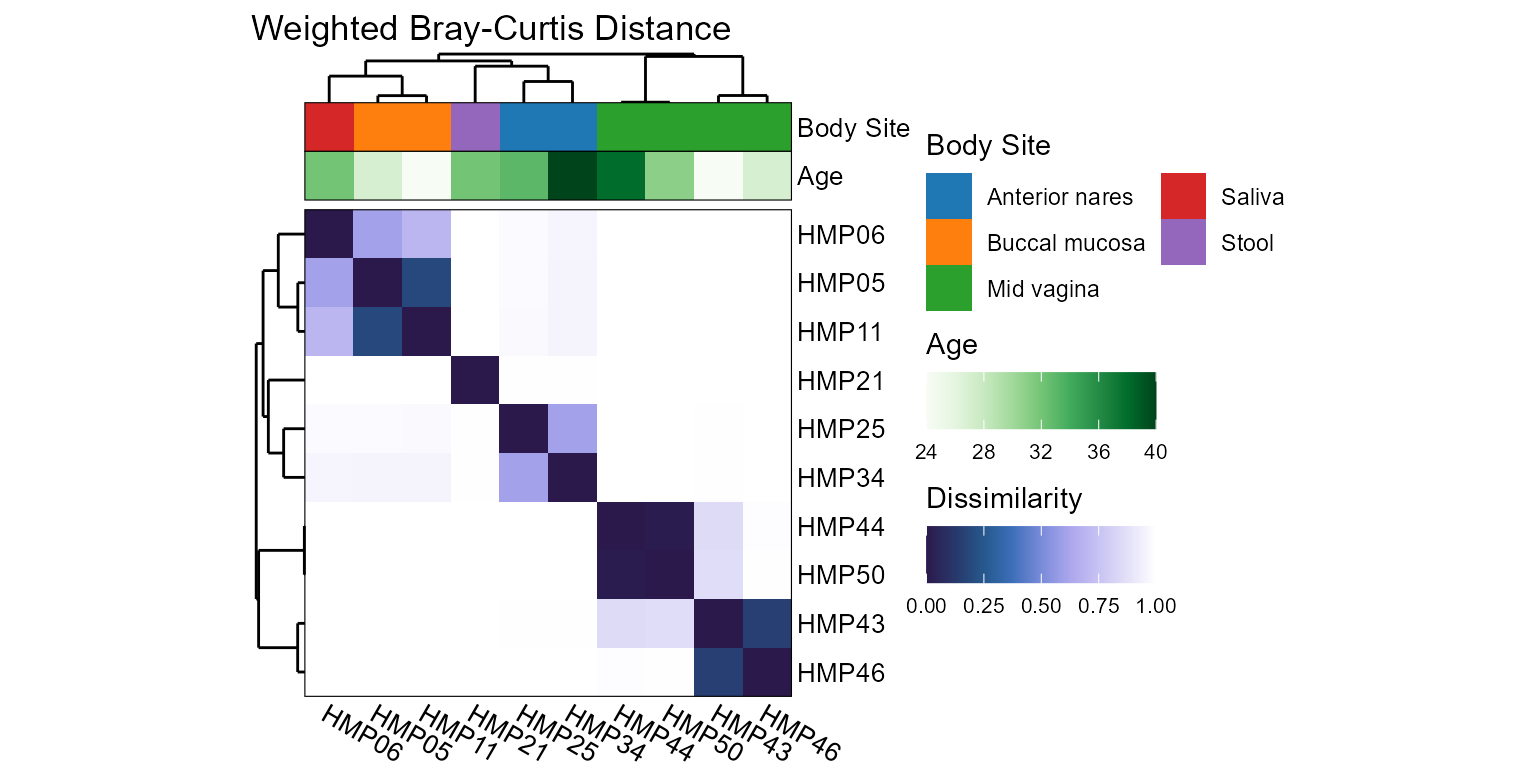
## Categorical ----------------------------
tracks = "Body Site"
tracks = list('Body Site' = "bright")
tracks = list('Body Site' = c('Stool' = "blue", 'Saliva' = "green"))

## Numeric --------------------------------
tracks = "Age"
tracks = list('Age' = "reds")

## Multiple Tracks ------------------------
tracks = c("Body Site", "Age")
tracks = list('Body Site' = "bright", 'Age' = "reds")
tracks = list(
  'Body Site' = c('Stool' = "blue", 'Saliva' = "green"),
  'Age'       = list('colors' = "reds") )
The following entries in the track definitions are understood:
colors-A pre-defined palette name or custom set of colors to map to.
range-The c(min,max) to use for scale values.
label-Label for this track. Defaults to the name of this list element.
side-Options are
"top"(default) or"left".na.color-The color to use for
NAvalues.bins-Bin a gradient into this many bins/steps.
guide-A list of arguments for guide_colorbar() or guide_legend().
All built-in color palettes are colorblind-friendly.
Categorical palette names: "okabe", "carto", "r4",
"polychrome", "tol", "bright", "light",
"muted", "vibrant", "tableau", "classic",
"alphabet", "tableau20", "kelly", and "fishy".
Numeric palette names: "reds", "oranges", "greens",
"purples", "grays", "acton", "bamako",
"batlow", "bilbao", "buda", "davos",
"devon", "grayC", "hawaii", "imola",
"lajolla", "lapaz", "nuuk", "oslo",
"tokyo", "turku", "bam", "berlin",
"broc", "cork", "lisbon", "roma",
"tofino", "vanimo", and "vik".
See also
Other beta_diversity:
bdiv_boxplot(),
bdiv_clusters(),
bdiv_corrplot(),
bdiv_ord_plot(),
bdiv_ord_table(),
bdiv_stats(),
bdiv_table(),
distmat_stats()
Other visualization:
adiv_boxplot(),
adiv_corrplot(),
bdiv_boxplot(),
bdiv_corrplot(),
bdiv_ord_plot(),
plot_heatmap(),
rare_corrplot(),
rare_multiplot(),
rare_stacked(),
stats_boxplot(),
stats_corrplot(),
taxa_boxplot(),
taxa_corrplot(),
taxa_heatmap(),
taxa_stacked()