rbiom

Create

The general purpose as_rbiom() function can convert most data types into an rbiom object - see importing for details. Here we’ll import a dataset from a BIOM file.

library(rbiom)

file <- system.file(package = "rbiom", "extdata", "hmp50.bz2")
biom <- as_rbiom(file)

biom
#> Human Microbiome Project - 50 Sample Demo (2024-03-15)
#>      50 Samples:  HMP01, HMP02, HMP03, ..., and HMP50
#>     490 OTUs:     Unc01yki, Unc53100, LtbAci52, ...
#>       7 Ranks:    .otu, Kingdom, Phylum, ..., and Genus
#>       5 Metadata: .sample, Age, BMI, Body Site, and Sex
#>         Tree:     <present>

Inspect

The rbiom object has many helpful accessors.

Accessor	Content
`$counts`	Abundance of each OTU in each sample.
`$metadata`	Sample mappings to metadata (treatment, patient, etc).
`$taxonomy`	OTU mappings to taxonomic ranks (genus, phylum, etc).
`$otus`, `$n_otus`	OTU names.
`$samples`, `$n_samples`	Sample names.
`$fields`, `$n_fields`	Metadata field names.
`$ranks`, `$n_ranks`	Taxonomic rank names.
`$tree`, `$sequences`	Phylogenetic tree / sequences for the OTUs, or `NULL`.
`$id`, `$comment`	Arbitrary strings for describing the dataset, or `""`.
`$depth`	Rarefaction depth, or `NULL` if unrarefied.

biom$counts[1:4,1:8] %>% as.matrix()
#>          HMP01 HMP02 HMP03 HMP04 HMP05 HMP06 HMP07 HMP08
#> Unc01yki     0     0     0     0     0     0     0     0
#> Unc53100  1083   543   301   223  2672   748  2436   321
#> LtbAci52     0     0     0     0     0     0     0     0
#> CnbTube3     0     0     0     0     0     0     0     0

biom$fields
#> [1] ".sample"   "Age"       "BMI"       "Body Site" "Sex"

# Use pull() to automatically setNames().
pull(biom, 'Age') %>% head()
#> HMP01 HMP02 HMP03 HMP04 HMP05 HMP06 
#>    22    24    28    25    27    32

pull(), sample_sums(), taxa_matrix(), taxa_means(), taxa_sums()

Clone

Rbiom objects are passed by reference. The common <- assignment operator creates a second reference to the same object - it does not create a second object. To create a copy of an rbiom object, use the object’s $clone() method.

a <- as_rbiom(file)
b <- a$clone()  # Correct

a$n_samples
#> [1] 50
b$metadata %<>% head()
a$n_samples
#> [1] 50

a <- as_rbiom(file)
b <- a  # Wrong

a$n_samples
#> [1] 50
b$metadata %<>% head()
a$n_samples
#> [1] 6

Modify

There are seven components of an rbiom object which you can modify directly. Assigning new values to these components will trigger validation checks and inter-component OTU/sample synchronization. See Working with rbiom Objects for additional details.

Component	What can be assigned.
`$counts`	matrix of abundances; OTUs (rows) by samples (columns)
`$metadata`	data.frame with `'.sample'` as the first column
`$taxonomy`	data.frame with `'.otu'` as the first column
`$tree`	phylo object with the phylogenetic tree for OTUs
`$sequences`	character vector of reference sequences for OTUs
`$id`	string with a title for the dataset
`$comment`	string with additional information about the dataset

Rarefy Counts

A common way to normalize microbiome count data is to rarefy it. This process drops samples with too few observations, and randomly removes observations from the remaining samples, so that all samples have the same “rarefaction depth”.

sample_sums(biom) %>% head()
#> HMP01 HMP02 HMP03 HMP04 HMP05 HMP06 
#>  1660  1371  1353  1895  3939  4150

biom <- rarefy(biom)

sample_sums(biom) %>% head()
#> HMP01 HMP02 HMP03 HMP04 HMP05 HMP06 
#>  1183  1183  1183  1183  1183  1183

Add Metadata

Additional sample metadata columns can be added to biom$metadata (a tibble data.frame). The first column, '.sample', is used by rbiom to link sample metadata to samples in the abundance table.

biom$metadata$group <- sample(c('A', 'B'), biom$n_samples, TRUE)
biom %<>% mutate(Obese = BMI >= 30, Sex = NULL)
biom %<>% rename('Years Old' = "Age")
biom$metadata
#> # A tibble: 49 × 6
#>   .sample `Years Old`   BMI `Body Site`   group Obese
#>   <chr>         <dbl> <dbl> <fct>         <fct> <lgl>
#> 1 HMP01            22    20 Buccal mucosa A     FALSE
#> 2 HMP02            24    23 Buccal mucosa B     FALSE
#> 3 HMP03            28    26 Saliva        A     FALSE
#> 4 HMP04            25    23 Saliva        B     FALSE
#> 5 HMP05            27    24 Buccal mucosa A     FALSE
#> # ℹ 44 more rows

mutate(), rename()

Subset Samples

Removing samples from the metadata will remove those samples from the entire rbiom object.

biom %<>% subset(`Body Site` == "Anterior nares")
biom$metadata
#> # A tibble: 10 × 6
#>   .sample `Years Old`   BMI `Body Site`    group Obese
#>   <chr>         <dbl> <dbl> <fct>          <fct> <lgl>
#> 1 HMP10            22    20 Anterior nares B     FALSE
#> 2 HMP15            25    21 Anterior nares A     FALSE
#> 3 HMP16            24    19 Anterior nares B     FALSE
#> 4 HMP25            33    32 Anterior nares B     TRUE 
#> 5 HMP31            31    20 Anterior nares A     FALSE
#> # ℹ 5 more rows
biom
#> Human Microbiome Project - 50 Sample Demo (2024-03-15)
#>      10 Samples:  HMP10, HMP15, HMP16, ..., and HMP48
#>     126 OTUs:     CnbTube3, PpbAcne6, Unc02qsf, ...
#>       7 Ranks:    .otu, Kingdom, Phylum, ..., and Genus
#>       6 Metadata: .sample, Years Old, BMI, ..., and Obese
#>         Tree:     <present>

subset(), slice()

Compute

Functions that end in _table or _matrix return calculation results for use outside of rbiom. The _table suffix indicates the returned object will be a tibble data.frame with one computed value per row. Alternatively, _matrix will return a base R matrix.

taxa_table(biom, rank = "Phylum")
#> # A tibble: 80 × 9
#>   .rank  .sample .taxa      .abundance `Years Old`   BMI `Body Site` group Obese
#>   <fct>  <chr>   <fct>           <dbl>       <dbl> <dbl> <fct>       <fct> <lgl>
#> 1 Phylum HMP10   Actinobac…        676          22    20 Anterior n… B     FALSE
#> 2 Phylum HMP10   Bacteroid…          7          22    20 Anterior n… B     FALSE
#> 3 Phylum HMP10   Cyanobact…          0          22    20 Anterior n… B     FALSE
#> 4 Phylum HMP10   Deinococc…          0          22    20 Anterior n… B     FALSE
#> 5 Phylum HMP10   Firmicutes        496          22    20 Anterior n… B     FALSE
#> # ℹ 75 more rows

taxa_matrix(biom, rank = "Phylum")[1:4, 1:8]
#>                     HMP10 HMP15 HMP16 HMP25 HMP31 HMP32 HMP34 HMP40
#> Actinobacteria        676   862   648   442   670   606  1031   879
#> Bacteroidetes           7     2     2     0    79    20    15     0
#> Cyanobacteria           0     0     2     0     0    23     0     0
#> Deinococcus Thermus     0     0     0     0     0     1     0     0

Functions for taxa abundance (like the above taxa_table()) are prefixed by taxa_. Similarly, adiv_ is used for alpha diversity and bdiv_ for beta diversity.

adiv_matrix(), adiv_table(), bdiv_table(), bdiv_ord_table(), taxa_table(), taxa_matrix()

Visualize

The plotting functions in rbiom make it easy to produce informative visualizations about alpha diversity, beta diversity, and taxa abundance, and explore associations between those metrics and sample metadata.

See the Plot Types article for an overview of all the different plot options, and Mapping Metadata to Aesthetics for guidance on using colors, shapes, and patterns to represent metadata values.

For example, to display an ordination colored by body site:

bdiv_ord_plot(biom = hmp50, color.by = "Body Site")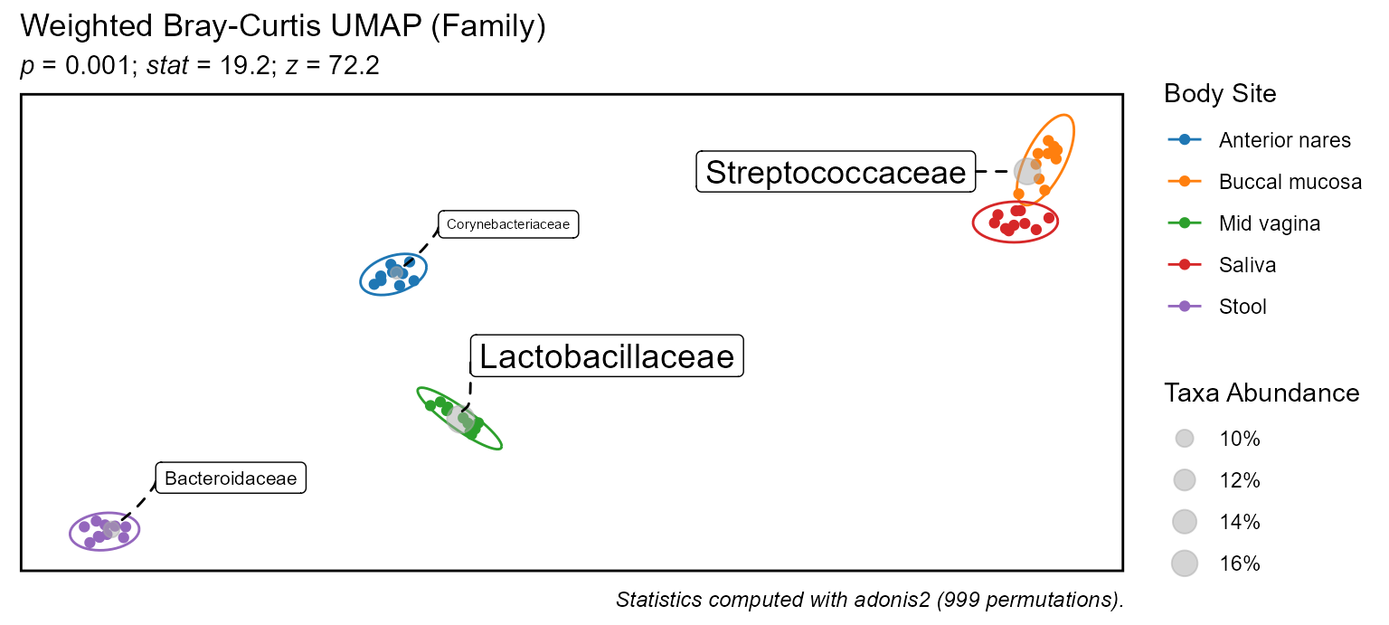

adiv_boxplot(), adiv_corrplot(), bdiv_boxplot(), bdiv_corrplot(), bdiv_heatmap(), bdiv_ord_plot(), rare_stacked(), rare_corrplot(), rare_multiplot(), taxa_stacked(), taxa_boxplot(), taxa_corrplot(), taxa_heatmap()

Analyze

Visualizations are an excellent way to observe differences between sample groups. When color.by is set, boxplots, corrplots, and ord_plots will include the following:

p-values and brief methodology on the plot itself.
$stats attribute with a detailed statistics table.
$stats$code attribute with the R code used to generate the table.

The Statistics article reviews this topic in greater detail.

p <- adiv_boxplot(hmp50, color.by = "Body Site", facet.by = "Sex")
p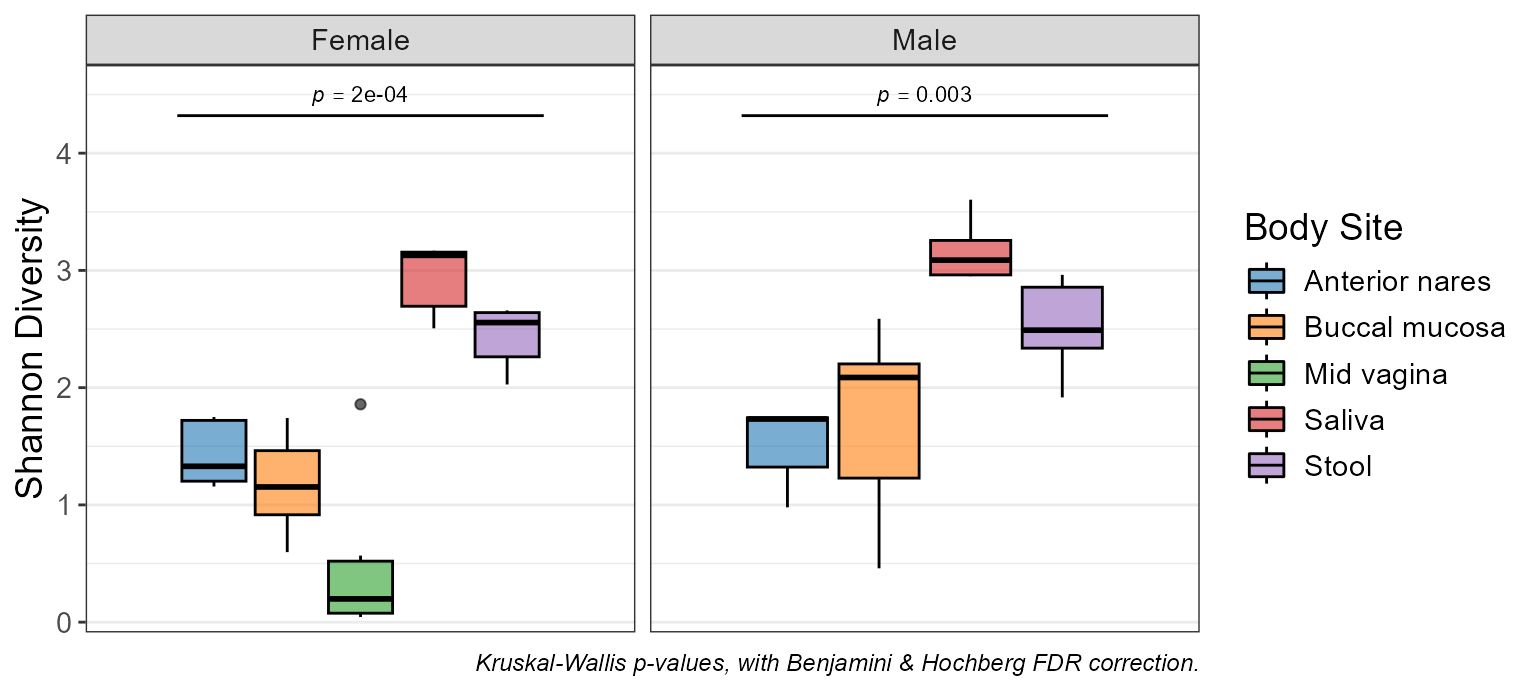

p$stats
#> # Test:     kruskal.test(.diversity ~ `Body Site`).
#> # A tibble: 2 × 6
#>   Sex       .n .stat   .df    .p.val   .adj.p
#>   <fct>  <int> <dbl> <int>     <dbl>    <dbl>
#> 1 Female    30  24.1     4 0.0000761 0.000152
#> 2 Male      20  13.9     3 0.00302   0.00302

p$stats$code
#> data  <- adiv_table(biom)
#> stats <- plyr::ddply(data, "Sex", function (d) {
#>   
#>   stats::kruskal.test(.diversity ~ `Body Site`, data = d) %>%
#>       
#>     with(data.frame(
#>       row.names = NULL, 
#>       .n     = nrow(d), 
#>       .stat  = statistic, 
#>       .df    = parameter, 
#>       .p.val = p.value )) %>%
#>       
#>     tryCatch(error = function (e) data.frame()[1,])
#>   
#> })

adiv_stats(), bdiv_stats(), distmat_stats(), taxa_stats()

Plots are essentially ggplot objects, and ggplot2::ggsave() can save them as PNG, PDF, SVG, and many other image file types.

To save your rbiom object to a BIOM file, use write_biom(). When sharing a dataset with someone who is unfamiliar with accessing BIOM files, write_xlsx() is also an option.

A few additional resources to know about:

R Markdown - reproducible analyses/reports.
flexdashboard - interactive dashboards.
atima - rbiom in website form.

ggplot2::ggsave(), patchwork::wrap_plots(), write_biom(), write_xlsx()