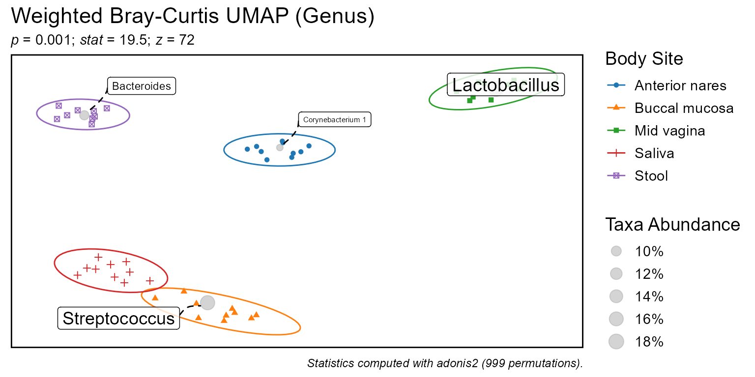
Ordinate samples and taxa on a 2D plane based on beta diversity distances.
Source:R/bdiv_ord_plot.r
bdiv_ord_plot.RdOrdinate samples and taxa on a 2D plane based on beta diversity distances.
Usage
bdiv_ord_plot(
  biom,
  bdiv = "bray",
  ord = "PCoA",
  layers = "petm",
  stat.by = NULL,
  facet.by = NULL,
  colors = TRUE,
  shapes = TRUE,
  tree = NULL,
  test = "adonis2",
  seed = 0,
  permutations = 999,
  rank = -1,
  taxa = 4,
  p.top = Inf,
  p.adj = "fdr",
  unc = "singly",
  caption = TRUE,
  alpha = 0.5,
  cpus = n_cpus(),
  ...
)
Arguments
- biom
An rbiom object, or any value accepted by
as_rbiom().- bdiv
Beta diversity distance algorithm(s) to use. Options are:
c("aitchison", "bhattacharyya", "bray", "canberra", "chebyshev", "chord", "clark", "sorensen", "divergence", "euclidean", "generalized_unifrac", "gower", "hamming", "hellinger", "horn", "jaccard", "jensen", "jsd", "lorentzian", "manhattan", "matusita", "minkowski", "morisita", "motyka", "normalized_unifrac", "ochiai", "psym_chisq", "soergel", "squared_chisq", "squared_chord", "squared_euclidean", "topsoe", "unweighted_unifrac", "variance_adjusted_unifrac", "wave_hedges", "weighted_unifrac"). For the UniFrac family, a phylogenetic tree must be present inbiomor explicitly provided viatree=. Supports partial matching. Multiple values are allowed for functions which return a table or plot. Default:"bray"- ord
Method for reducing dimensionality. Options are:
"PCoA"-Principal coordinate analysis;
ape::pcoa()."UMAP"-Uniform manifold approximation and projection;
uwot::umap()."NMDS"-Nonmetric multidimensional scaling;
vegan::metaMDS()."tSNE"-t-distributed stochastic neighbor embedding;
tsne::tsne().
Multiple/abbreviated values allowed. Default:
"PCoA"- layers
One or more of
c("point", "spider", "ellipse", "name", "mean", "taxon", "arrow"). The first four are sample-centric; the last three are taxa-centric. Single letter abbreviations are also accepted. For instance,c("point", "ellipse")is equivalent toc("p", "e")and"pe". Default:"pe"- stat.by
The categorical or numeric metadata field over which statistics should be calculated. Required.
- facet.by
Dataset field(s) to use for faceting. Must be categorical. Default:
NULL- colors
How to color the groups. Options are:
TRUE-Automatically select colorblind-friendly colors.
FALSEorNULL-Don't use colors.
- a palette name -
Auto-select colors from this set. E.g.
"okabe"- character vector -
Custom colors to use. E.g.
c("red", "#00FF00")- named character vector -
Explicit mapping. E.g.
c(Male = "blue", Female = "red")
See "Aesthetics" section below for additional information. Default:
TRUE- shapes
Shapes for each group. Options are similar to
colors's:TRUE,FALSE,NULL, shape names (typically integers 0 - 17), or a named vector mapping groups to specific shape names. See "Aesthetics" section below for additional information. Default:TRUE- tree
A
phyloobject representing the phylogenetic relationships of the taxa inbiom. Only required when computing UniFrac distances. Default:biom$tree- test
Permutational test for accessing significance. Options are:
"adonis2"-Permutational MANOVA;
vegan::adonis2()."mrpp"-Multiple response permutation procedure;
vegan::mrpp()."none"-Don't run any statistics.
Abbreviations are allowed. Default:
"adonis2"- seed
Random seed for permutations. Must be a non-negative integer. Default:
0- permutations
Number of random permutations to use. Default:
999- rank
What rank(s) of taxa to display. E.g.
"Phylum","Genus",".otu", etc. An integer vector can also be given, where1is the highest rank,2is the second highest,-1is the lowest rank,-2is the second lowest, and0is the OTU "rank". Runbiom$ranksto see all options for a given rbiom object. Default:-1.- taxa
Which taxa to display. An integer value will show the top n most abundant taxa. A value 0 <= n < 1 will show any taxa with that mean abundance or greater (e.g.
0.1implies >= 10%). A character vector of taxa names will show only those named taxa. Default:6.- p.top
Only display taxa with the most significant differences in abundance. If
p.topis >= 1, then thep.topmost significant taxa are displayed. Ifp.topis less than one, all taxa with an adjusted p-value <=p.topare displayed. Recommended to be used in combination with thetaxaparameter to set a lower bound on the mean abundance of considered taxa. Default:Inf- p.adj
Method to use for multiple comparisons adjustment of p-values. Run
p.adjust.methodsfor a list of available options. Default:"fdr"- unc
How to handle unclassified, uncultured, and similarly ambiguous taxa names. Options are:
"singly"-Replaces them with the OTU name.
"grouped"-Replaces them with a higher rank's name.
"drop"-Excludes them from the result.
"asis"-To not check/modify any taxa names.
Abbreviations are allowed. Default:
"singly"- caption
Add methodology caption beneath the plot. Default:
TRUE- alpha
The alpha term to use in Generalized UniFrac. How much weight to give to relative abundances; a value between 0 and 1, inclusive. Setting
alpha=1is equivalent to Normalized UniFrac. Default:0.5- cpus
The number of CPUs to use. Set to
NULLto use all available, or to1to disable parallel processing. Default:NULL- ...
Parameters for layer geoms (e.g.
ggplot2::geom_point()). Prefixing parameter names with a layer name ensures that a particular parameter is passed to, and only to, that layer. For instance,point.size = 2orp.size = 2ensures only the points have their size set to2. Points can also be controlled with thept.prefix.
Value
A ggplot2 plot.
The computed sample coordinates and ggplot command
are available as $data and $code respectively.
If stat.by is given, then $stats and
$stats$code are set.
If rank is given, then $data$taxa_coords,
$taxa_stats, and $taxa_stats$code are set.
See also
Other beta_diversity:
bdiv_boxplot(),
bdiv_clusters(),
bdiv_corrplot(),
bdiv_heatmap(),
bdiv_ord_table(),
bdiv_stats(),
bdiv_table(),
distmat_stats()
Other ordination:
bdiv_ord_table(),
distmat_ord_table()
Other visualization:
adiv_boxplot(),
adiv_corrplot(),
bdiv_boxplot(),
bdiv_corrplot(),
bdiv_heatmap(),
plot_heatmap(),
rare_corrplot(),
rare_multiplot(),
rare_stacked(),
stats_boxplot(),
stats_corrplot(),
taxa_boxplot(),
taxa_corrplot(),
taxa_heatmap(),
taxa_stacked()
