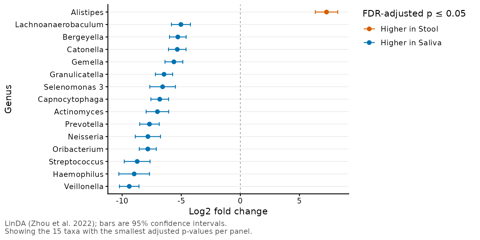
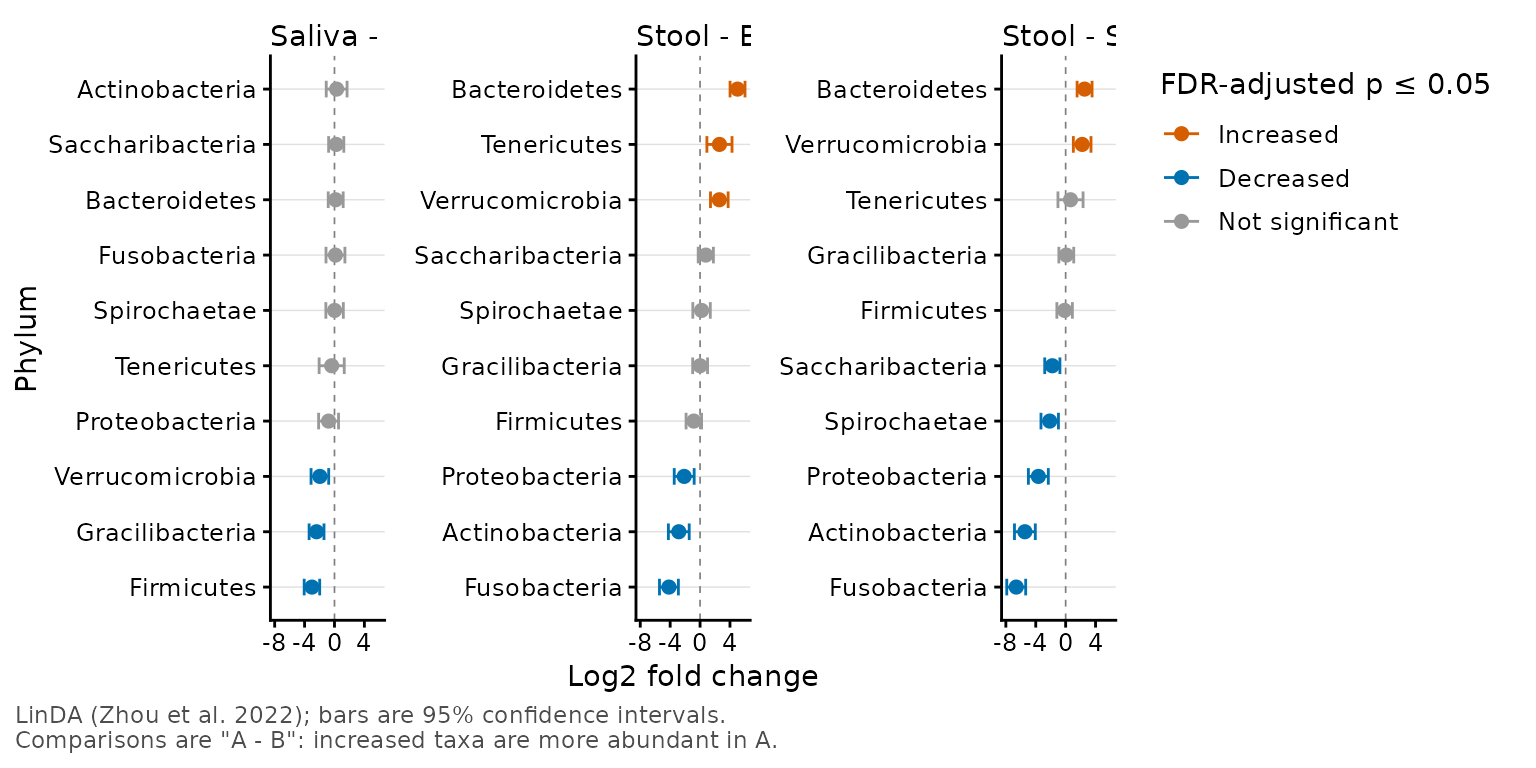
Plot differential abundance as a forest plot.

Runs taxa_da() and shows each taxon's log2 fold change as a point with its confidence interval. Significant taxa are colored by the direction of the change; the others are gray. Each comparison (and rank and split.by subset) gets its own panel, with the taxa ordered by fold change.

Usage

taxa_forest(
  biom,
  stat.by = NULL,
  regr = NULL,
  rank = -1,
  taxa = NULL,
  method = "linda",
  covariates = NULL,
  split.by = NULL,
  strata = NULL,
  p.top = 20,
  p.sig = 0.05,
  colors = TRUE,
  caption = TRUE,
  prev.cut = 0.1,
  level = 0.95,
  p.adj = "fdr",
  lineage = FALSE,
  unc = "singly",
  ...
)

Arguments

biom

An rbiom object, or any value accepted by as_rbiom().

stat.by

Dataset field with the groups to compare. Must be categorical. Each pair of groups is compared, in the order of the field's levels: with levels A, B, and C, the comparisons are "B - A", "C - A", and "C - B", and a positive log fold change means the taxon is more abundant in the first-named group. Give either stat.by or regr, not both. Default: NULL

regr

Dataset field with a numeric variable. The log fold change is then per unit increase in regr. Give either stat.by or regr, not both. Default: NULL

rank

What rank(s) of taxa to test. E.g. "Phylum", "Genus", ".otu", etc. An integer vector can also be given, where 1 is the highest rank, -1 is the lowest rank, and 0 is the OTU "rank". Each rank is analyzed separately. Default: -1

taxa

Which taxa to report. An integer value reports the top n most abundant taxa, a value 0 <= n < 1 reports the taxa with that mean relative abundance or greater, and a character vector reports the named taxa. Every taxon that passes prev.cut is still part of the analysis, since LinDA estimates the compositional bias from all of them, and p-values are adjusted for all of them. Default: NULL (all tested taxa).

method

The differential abundance method. Currently only "linda". See Details. Default: "linda"

covariates

Dataset field(s) to adjust for, such as age or antibiotic use. They are included in every model, but their own effects are not reported. Default: NULL

split.by

Dataset field(s) that the samples should be split by. Each subset is analyzed separately. Must be categorical. Default: NULL

strata

Dataset field with a blocking variable, such as a subject identifier for repeated measures. Must be categorical. Adds a random intercept per stratum to every model, fitted as linear mixed models with lmerTest::lmer() (requires the lmerTest package). Default: NULL

p.top

Which taxa to show in each panel. A value >= 1 shows the p.top taxa with the smallest adjusted p-values; a value < 1 shows the taxa with an adjusted p-value <= p.top; Inf shows every tested taxon. Default: 20

p.sig

Taxa with an adjusted p-value <= p.sig are significant and colored by the direction of the change. Default: 0.05

colors

Colors for significant taxa that are more abundant in the first-named group of the comparison (or that increase with regr), for those that are less abundant (or decrease), and for taxa that aren't significant, in that order. Two colors use the default gray for the third. TRUE uses vermillion, blue, and gray; a palette name (e.g. "okabe") uses its first two colors; FALSE draws everything in black. Default: TRUE

caption

Add a caption describing the method, the intervals, and which taxa are shown. Default: TRUE

prev.cut

Prevalence filter: taxa found in fewer than this proportion of the samples are not tested. Default: 0.1

level

The confidence level for the confidence intervals (.lower and .upper). Default: 0.95

p.adj

Method to use for multiple comparisons adjustment of p-values. Run p.adjust.methods for a list of available options. As is standard for differential abundance, p-values are adjusted across taxa separately for each comparison (and each rank and split.by subset). Default: "fdr"

lineage

Include all ranks in the name of the taxa. For instance, setting to TRUE will produce Bacteria; Actinobacteria; Coriobacteriia; Coriobacteriales. Otherwise the taxa name will simply be Coriobacteriales. You want to set this to TRUE when unc = "asis" and you have taxa names (such as Incertae_Sedis) that map to multiple higher level ranks. Default: FALSE

unc

How to handle unclassified, uncultured, and similarly ambiguous taxa names. Options are:

"singly" -: Replaces them with the OTU name.
"grouped" -: Replaces them with a higher rank's name.
"drop" -: Excludes them from the result.
"asis" -: To not check/modify any taxa names.

Abbreviations are allowed. Default: "singly"

...

Parameters for the underlying ggplot2 functions. Prefix a parameter with a layer name to pass it to that layer only: point. (ggplot2::geom_point()), ci. (ggplot2::geom_errorbar(); e.g. ci.width = 0 for no caps), zero. (the ggplot2::geom_vline() at zero), facet., labs., xaxis., yaxis., and theme.. An argument that no layer accepts is an error.

Value

A ggplot2 plot. The computed data points and ggplot command are available as $data and $code, respectively.

Details

The statistics are those of taxa_da(), which is called with the same arguments; they are available as $stats, and the code that reproduces the plot as $code. Each panel shows its own taxa (p.top), so the y-axes are independent. To keep a taxon's position unique within its panel, the plotted y values are the row number and taxon name (e.g. "12-Bacteroides"); the axis labels drop the row number.

Examples

    library(rbiom)

    biom <- subset(hmp50, `Body Site` %in% c("Saliva", "Stool"))
    taxa_forest(biom, stat.by = "Body Site", rank = "Genus", p.top = 15)


    biom <- subset(hmp50, `Body Site` %in% c("Saliva", "Stool", "Buccal mucosa"))
    taxa_forest(biom, stat.by = "Body Site", rank = "Phylum", p.top = Inf)